One of the video games I’ve played the most in the past year or so is Slay the Spire. Since it’s getting out of early access next week (and getting more expensive 😉 ), I thought it’d be a good moment to write a few words about it.
Slay the Spire is described as “card game meets roguelike“. The exact qualification of “roguelike” is debatable, but oh well 😉 It works as follows: you start with a character with a basic deck of cards. You enter a randomly generated dungeon – with a few constraints in the rooms you can actually encounter. For each room, you either have a fight, a merchant, a resting place, a treasure, or a random encounter that may or may not be to your benefit.
The fights are turn-based combats in which you play cards – either offensive or defensive. To play cards, you need to play their mana cost – you get, by default, 3 mana per turn (and the cards have integer costs 😉 ). At each round, you get at least an idea of what your enemy is going to inflict on you – including an exact number and strength of attacks – which allows you to make decisions on which compromise to make on that turn. Moreover, the enemies themselves are mostly deterministic: with a bit of play, you start knowing what’s in front of you and how you can beat them. The fight is over when either you or your opponent is defeated. If you are defeated, it’s game over: you’ll have to start a new dungeon run. When you win a fight, you get to add a new card (typically chosen between three) to add to your deck. When you win an elite fight, you also get to add a relic, which gives effects that stays between fights.
The game is split into three “acts”, all ending with an act boss, and the acts are getting tougher and tougher – but since you keep improving your deck and getting relics, it’s supposed to balance – if you play well, that is 😉
When you first start playing the game, you’ll need to unlock most of the features: cards, relics, characters. I don’t know if I’m too fond of the approach: on the one hand, it allows to get to know the possible cards and relics with a bit of time, which may help with the learning curve, and unlocking new content is fun; on the other hand, I remember being a bit frustrated by the speed of the unlocking.
The amount of content is pretty impressive. For the normal mode, there are three characters, each with their own cards and abilities. For each of these characters, you can unlock up to 20 “ascension modes”, which make the game harder and harder. And since the game is randomized, every game is a new challenge. (And yes, there’s a way to save a seed and to re-try a run.)
There are also two “special” modes: a “daily climb”, to which modifiers are applied and all the players can compete for the highest score, and a “custom” mode, where you can create your own set of modifiers to have fun with the engine. And I was just made aware of the amount of mods that this games has – including new playable characters – I think I’m doomed.
The annoying thing is that I’m still a fairly bad player. I played, according to the statistics, 200 hours; that gave me 36 victories and 204 deaths 😛 And I’m nowhere near running in the later ascension levels (I think I reached ascension 3 on one of the characters?). It’s a challenging game – and it’s, for me, really not easy to consistently create a reasonable deck, considering the randomness of the cards that can appear. The good thing is that a run is between 40 minutes and an hour, which is a fairly low time commitment (and, more importantly: a bounded one), especially since it can be split easily between rooms.
Overall, it’s a very solid game, and one that I continue playing. The community has some very nice things going on, there’s a lot of fan artwork, a statistics database, speed runs – you name it. The development has been very active during the whole “early access” duration, typically with an update a week, a lot of tweaking, re-balancing, and patch notes to which I looked forward every week. And any game that gives me 200+h of game play is definitely worth the money 🙂 Oh, and it runs on Linux 😀
Note: this is a translation with some re-writing of a previously published post: Le problème SAT.
I’m going to explain what the SAT problem is, because I’m going to talk about it a bit more soon. It’s one of the fundamental blocks around the P vs NP question; I’m going to write a blog post about NP-hard problems, but writing a post about SAT specifically is worth it. Also: I did my master thesis on SAT-related questions, so it’s a bit of a favorite topic of mine 🙂
SAT is a common abbreviation for “boolean satisfiability problem”. Everything revolves around the concept of boolean formulas, and a boolean formula can look like this:
Let me unpack this thing. The first concept is variables: here, , or . They’re kind of like the “unknowns” of an equation: we want to find values for , and . Moreover, we’re in a somewhat weird universe, the boolean universe: the only values , and can take are 0 or 1.
Then, we have some weird symbols. means “or”, and means “and”. And the small bars above some of the letters indicate a negation. We combine these symbols with variables to get expressions, whose value can be computed as follow:
If , then , otherwise ( is the opposite value of ). We read this “not “.
If , then ; if , then ; if and , then . In other words, if or . Note that in this context, when we say “or”, we do not use exactly the same meaning than in everyday language: we mean “if or if or if both are equal to 1″. We read this: “ or “.
If and , then , otherwise . We read this: “ and “.
I’m summarizing all this in this table, for every possible value of and :
We can combine these expressions any way that we want to get boolean formulas. So the following examples are boolean formulas:
And then, by assigning values (0 or 1) to the individual variables, we can evaluate a formula for the assignment, that is to say, say if the value that the formula “computes” is 0 or 1. If the formula evaluates to 1 with an assignment, we say that this assignment satisfies the formula. And we say that a formula is satisfiable if there exists an assignment that makes it evaluate to 1 – hence the name of the problem, “boolean satisfiability”.
Boolean satisfiability in general is kind of “annoying” because it doesn’t have much structure to it: it’s hard to think about and it’s hard to say much about it, really. One thing that is always feasible, however, is to look at all the possibilities for all the variables, and see if there exists a combination of values that satisfies the formula. Picking one of the example above, and calling the formula :
And let’s enumerate all possibilities:
This table answers the question “is there values of , and for which evaluates to 1 (the answer is yes) and it even goes further by giving said values (for instance, , and are values that satisfy the formula).
The issue is that it’s not really manageable to write such a table as soon as we get a lot of variables. The reason for that is that, for every variable, I need to check what happens for its 0 value and for its 1 value. So I have two choices for the first variable, two choices for the second variable, two choices for the third variable, and so on. The choices multiply with each other: similarly to the table above, I need a line for every possible combination of values of variables. For 3 variables, lines. For 5 variables, lines, that starts to be annoying to do by hand. For 20 variables, lines, the result is not necessarily instant anymore on a computer. And it continues growing: for variables, I need lines, which it grows faster and faster: the joys of power functions.
For the people who followed the previous explanations, this is NOT a polynomial time algorithm: it’s an exponential time algorithm. (Not even considering the fact that I’m only enumerating the possibilities and not evaluating the formula yet).
Since the general SAT problem seems fairly complicated to tackle, one can wonder if there are “subgroups” that are easy to solve, or that are easier to think about. And, indeed, there are such subgroups.
Suppose that, instead of getting an arbitrary combination of variables and symbols, I restrict myself of formulas such as this one: . That’s a form where I have “groups” of variables linked by ““, themselves grouped by . Then that’s an “easy” case: for the formula to be satisfiable, I only need one of the “groups” to evaluate to 1 (because they are linked by “or” operators, so the formula evaluates to 1 if at least one of the groups evaluates to 1). And a given group evaluates to 1, unless it contains both one variable and its negation, like . In that case, since within a group I need all the variables to be equal to 1 for the group to evaluate to 1, and since a variable and its negation cannot be equal both to 1, the group would evaluate to 0. So unless all the groups contain a variable and its negation, the formula is satisfiable – a fairly easy condition to verify.
If I consider the “opposite” of the previous setup, with formulas such as , we have “groups” of variables linked by , themselves grouped by . This type of formulas are called CNF formulas (where CNF means “conjunctive normal form”). A CNF formula is defined as a set of clauses (the “groups”), all linked by symbols (“and”). A clause is a set of one or several literals that are linked by symbols (“or”). A literal is either a variable (for example ) or its negation (for example ).
The question asked by an instance of the SAT problem is “can I find values for all variables such that the whole formula evaluates to 1?”. If we restrict ourselves to CNF formulas (and call the restricted problem CNF-SAT), this means that we want that all the clauses evaluate to 1, because since they are linked by “and” in the formula, I need that all of its clauses evaluate to 1. And for each clause to have value 1, I need at least one of the literals to have value 1 in the clause (I want the first literal or the second literal or the third literal or… to be equal to 1). As previously mentioned: it can happen that all the literals are equal to 1 – the clause will still be equal to 1.
It turns out that we can again look at subgroups within CNF formulas. Let us consider CNF formulas that have exactly 2 literals in all clauses – they are called 2-CNF formulas. The associated problem is called 2-CNF-SAT, or more often 2-SAT. Well, 2-SAT can be solved in linear time. This means that there exists an algorithm that, given any 2-CNF formula, can tell in linear time whether the formula is satisfiable or not.
Conversely, for CNF formulas that have clauses that have more than 2 literals… in general, we don’t know. We can even restrict ourselves to CNF formulas that have exactly 3 literals in each clause and still not know. The associated problem is called 3-CNF-SAT, or (much) more often 3-SAT.
From a “complexity class” point of view, 3-SAT is in NP. If I’m given a satisfiable 3-CNF formula and values for all variables of the formula, I can check in polynomial time that it works: I can check that a formula is satisfiable if I have a proof of it. (This statement is also true for general SAT formulas.)
What we do not know, however, is whether 3-SAT is in P: we do not know if there exists a polynomial time algorithm that allows us to decide if a 3-CNF formula can be satisfied or not in the general case. The difficulty of the problem still does not presume of the difficulty of individual instances. In general, we do not know how to solve the 3-SAT problem; in practice, 3-SAT instances are solved every day.
We also do not know whether 3-SAT is outside of P: we do not know if we need an algorithm that is “more powerful” than a polynomial time algorithm to solve the problem in the general case. To answer that question (and to prove it) would actually allow to solve the P vs NP problem – but to explain that, I need to explain NP-hard problems, and that’s something for the next post, in which I’ll also explain why it’s pretty reasonable to restrict oneself to 3-SAT (instead of the general SAT problem) when it comes to studying the theory of satisfiability 🙂
I used to gather some “cool stuff from the Internet” a long, long time ago on my French blog. Since then, that sort of “content gathering” has mostly been moved to social networks; let’s see if I can put that back in blog form instead. This could actually be a nice Friday post 🙂
Modern Mrs Darcy’s 2019 Reading Challenge – I discovered MMD late last year, and I quite like what she does, even though we don’t necessarily have much in common (so far?) literature-wise. The Reading Challenge seems pretty fun, so I’ll try to tick the boxes this year.
To Wash It All Away [text, PDF] – an hilarious piece by James Mickens (yeah, the same one as in the video of the first link) about the terrible, terrible state of web technologies. It’s awfully mean, but delightfully and well-writtenly so.
Orders of Magnitude [image] and Observable universe logarithmic illustration [image] – some very pretty illustrations of the universe (one in layers at different scales, one in logarithmic scale) from Pablo Carlos Budassi, taken from the article above.
Gygax – 2nd Edition Review [text, music] – a review of one of my favorite albums this year – and actually the review that made me listen to it in the first place. GUYS: IT’S D&D METAL. IT’S BRILLIANT. The only annoying thing is that it tends to make me dance at my desk more often than other albums.
The Hot New Asset Class Is Lego Sets [text] – if you need an excuse to buy LEGO, you can just say it’s a way to diversify your portfolio, ‘cuz Bloomberg said so. Or you can just buy LEGO for the sake of it.
For Christmas, I got a crystal ball to use for photography. On Tuesday, the weather was nice, so I went in the city to experiment a bit with it.
First, I went to Lindenhof to get a re-take on my favorite view of the city.
The other side of that view is cool too:
Then I accidentally left my polarizing filter on – but that’s actually pretty cool, look, I’m holding a soap bubble!
And actually, photographing trees through that ball is pretty fun. But hey – I do have a favorite tree in Zürich! What if I visited it? A short tram ride later, here I am – Zürichhorn!
After a few more shots in the vicinity, I found another cool tree when walking back along the lake.
As I walked back to Bellevue, the night fell. Time to take a last one – I did not intend for the whole thing to be out of focus, but I happen to really like the end result 🙂
All right, I think I explained enough algorithmic complexity (part 1 and part 2) to start with a nice piece, which is to explain what is behind the “Is P equal to NP?” question – also called “P vs NP” problem.
The “P vs NP” problem is one of the most famous open problems, if not the most famous. It’s also part of the Millenium Prize problems, a series of 7 problems stated in 2000: anyone solving one of these problems gets awarded one million dollars. Only one of these problems has been solved, the Poincaré conjecture, proven by Grigori Perelman. He was awarded the Fields medal (roughly equivalent to a Nobel Prize in mathematics) for it, as well as the aforementioned million dollars; he declined both.
But enough history, let’s get into it. P and NP are called “complexity classes”. A complexity class is a set of problems that have common properties. We consider problems (for instance “can I go from point A to point B in my graph with 15 steps or less?”) and to put them in little boxes depending on their properties, in particularity their worst case time complexity (how much time do I need to solve them) and their worst case space complexity (how much memory do I need to solve them).
I explained in the algorithmic complexity blog posts what it meant for an algorithm to run in a given time. Saying that a problem can be/is solved in a given time means that we know how to solve it in that time, which means we have an algorithm that runs in that time and returns the correct solution. To go back to my previous examples, we saw that it was possible to sort a set of elements (books, or other elements) in time . It so happens that, in classical computation models, we can’t do better than . We say that the complexity of sorting is , and we also say that we can sort elements in polynomial time.
A polynomial time algorithm is an algorithm that finishes with a number of steps that is less than , where is the size of the input and an arbitrary number (including very large numbers, as long as they do not depend on ). The name comes from the fact that functions such as , , and are called polynomial functions. Since I can sort elements in time , which is smaller than , sorting is solved in polynomial time. It would also work if I could only sort elements in time , that would also be polynomial. The nice thing with polynomials is that they combine very well. If I make two polynomial operations, I’m still in polynomial time. If I make a polynomial number of polynomial operations, I’m still in polynomial time. The polynomial gets “bigger” (for instance, it goes from to ), but it stays a polynomial.
Now, I need to explain the difference between a problem and an instance of a problem – because I kind of need that level of precision 🙂 A problem regroups all the instances of a problem. If I say “I want to sort my bookshelf”, it’s an instance of the problem “I want to sort an arbitrary bookshelf”. If I’m looking at the length shortest path between two points on a given graph (for example a subway map), it’s an instance of the problem “length of shortest path in a graph”, where we consider all arbitrary graphs of arbitrary size. The problem is the “general concept”, the instance is a “concrete example of the general problem”.
The complexity class P contains all the “decision” problems that can be solved in polynomial time. A decision problem is a problem that can be answered by yes or no. It can seem like a huge restriction: in practice, there are sometimes way to massage the problem so that it can get in that category. Instead of asking for “the length of the shortest path” (asking for the value), I can ask if there is “a path of length less than X” and test that on various X values until I have an answer. If I can do that in a polynomial number of queries (and I can do that for the shortest path question), and if the decision problem can be solved in polynomial time, then the corresponding “value” problem can also be solved in polynomial time. As for an instance of that shortest path decision problem, it can be “considering the map of the Parisian subway, is there a path going from La Motte Piquet Grenelle to Belleville that goes through less than 20 stations?” (the answer is yes) or “in less than 10 stations?” (I think the answer is no).
Let me give another type of a decision problem: graph colorability. I like these kind of examples because I can make some drawings and they are quite easy to explain. Pick a graph, that is to say a bunch of points (vertices) connected by lines (edges). We want to color the vertices with a “proper coloring”: a coloring such that two vertices that are connected by a single edge do not have the same color. The graph colorability problems are problems such as “can I properly color this graph with 2, 3, 5, 12 colors?”. The “value” problem associated to the decision problem is to ask what is the minimum number of colors that I need to color the graph under these constraints.
Let’s go for a few examples – instances of the problem 🙂
A “triangle” graph (three vertices connected with three edges) cannot be colored with only two colors, I need three:
On the other hand, a “square-shaped” graph (four vertices connected as a square by four edges) can be colored with two colors only:
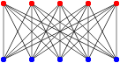
There are graphs with a very large number of vertices and edges that can be colored with only two colors, as long as they follow that type of structure:
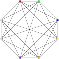
And I can have graphs that require a very large number of colors (one per vertex!) if all the vertices are connected to one another, like this:
And this is where it becomes interesting. We know how to answer in polynomial time (where is of the number of vertices of the graph) to the question “Can this graph be colored with two colors?” for any graph. To decide that, I color an arbitrary vertex of the graph in blue. Then I color all of its neighbors in red – because since the first one is blue, all of its neighbors must be red, otherwise we violate the constraint that no two connected vertices can have the same color. We try to color all the neighbors of the red vertices in blue, and so on. If we manage to color all the vertices with this algorithm, the graph can be colored with two colors – since we just did it! Otherwise, it’s because a vertex has a neighbor that constrains it to be blue (because the neighbor is red) and a neighbor that constrains it to be red (because the neighbor is blue). It is not necessarily obvious to see that it means that the graph cannot be colored with two colors, but it’s actually the case.
I claim that this algorithm is running in polynomial time: why is that the case? The algorithm is, roughly, traversing all the vertices in a certain order and coloring them as it goes; the vertices are only visited once; before coloring a vertex, we check against all of its neighbors, which in the worst case all the other vertices. I hope you can convince yourself that, if we do at most (number of vertices we traverse) times comparisons (maximum number of neighbors for a given vertex), we do at most operations, and the algorithm is polynomial. I don’t want to give much more details here because it’s not the main topic of my post, but if you want more details, ping me in the comments and I’ll try to explain better.
Now, for the question “Can this graph be colored with three colors?”, well… nobody has yet found a polynomial algorithm that allows us to answer the question for any instance of the problem, that is to say for any graph. And, for reasons I’ll explain in a future post, if you find a (correct!) algorithm that allows to answer that question in polynomial time, there’s a fair chance that you get famous, that you get some hate from the cryptography people, and that you win one million dollars. Interesting, isn’t it?
The other interesting thing is that, if I give you a graph that is already colored, and that I tell you “I colored this graph with three colors”, you can check, in polynomial time, that I’m not trying to scam you. You just look at all the edges one after the other and you check that both vertices of the edge are colored with different colors, and you check that there are only three colors on the graph. Easy. And polynomial.
That type of “easily checkable” problems is the NP complexity class. Without giving the formal definition, here’s the idea: a decision problem is in the NP complexity class if, for all instances for which I can answer “yes”, there exists a “proof” that allows me to check that “yes” in polynomial time. This “proof” allows me to answer “I bet you can’t!” by “well, see, I can color that way, it works, that proves that I can do that with three colors” – that is, if the graph is indeed colorable with 3 colors. Note here that I’m not saying anything about how to get that proof – just that if I have it, I can check that it is correct. I also do not say anything about what happens when the instance cannot be colored with three colors. One of the reasons is that it’s often more difficult to prove that something is impossible than to prove that it is possible. I can prove that something is possible by doing it; if I can’t manage to do something, it only proves that I can’t do it (but maybe someone else could).
To summarize:
P is the set of decision problems for which I can answer “yes” or “no” in polynomial time for all instances
NP is the set of decision problems for which, for each “yes” instance, I can get convinced in polynomial time that it is indeed the case if someone provides me with a proof that it is the case.
The next remark is that problems that are in P are also in NP, because if I can answer myself “yes” or “no” in polynomial time, then I can get convinced in polynomial time that the answer is “yes” if it is the case (I just have to run the polynomial time algorithm that answers “yes” or “no”, and to check that it answers “yes”).
The (literally) one-million-dollar question is to know whether all the problems that are in NP are also in P. Informally, does “I can see easily (i.e. in polynomial time) that a problem has a ‘yes’ answer, if I’m provided with the proof” also mean that “I can easily solve that problem”? If that is the case, then all the problems of NP are in P, and since all the problems of P are already in NP, then the P and NP classes contain exactly the same problems, which means that P = NP. If it’s not the case, then there are problems of NP that are not in P, and so P ≠ NP.
The vast majority of maths people think that P ≠ NP, but nobody managed to prove that yet – and many people try.
It would be very, very, very surprising for all these people if someone proved that P = NP. It would probably have pretty big consequences, because that would mean that we have a chance to solve problems that we currently consider as “hard” in “acceptable” times. A fair amount of the current cryptographic operations is based on the fact, not that it is “impossible” to do some operations, but that it’s “hard” to do them, that is to say that we do not know a fast algorithm to do them. In the optimistic case, proving that P = NP would probably not break everything immediately (because it would probably be fairly difficult to apply and that would take time), but we may want to hurry finding a solution. There are a few crypto things that do not rely on the hypothesis that P ≠ NP, so all is not lost either 😉
And the last fun thing is that, to prove that P = NP, it is enough to find a polynomial time algorithm for one of the “NP-hard” problems – of which I’ll talk in a future post, because this one is starting to be quite long. The colorability with three colors is one of these NP-hard problems.
I personally find utterly fascinating that a problem which is so “easy” to get an idea about have such large implications when it comes to its resolution. And I hope that, after you read what I just wrote, you can at least understand, if not share, my fascination 🙂
The theme for the second week of the 52Frames project was “Rule of Thirds“. I’ll admit my motivation for this theme was not very high – I considered going the “cheeky” route and take a picture of a third of a pie, but eh. And since it’s the second week, NOT submitting is inconceivable 😉
I knew motivation was going to be low, so when I went for lunch on Thursday and ran into that very pretty snowy tree, I took a bit of time to frame it within the constraints of said rule of thirds with my phone camera, thinking I’d have a backup shot in all cases.
I spent a bit of time doing some post-processing – cleaning up a few spots, removing a piece of road that was a bit ugly, and generally speaking bending the reality a little bit to get a better picture. Re-considering it right now, I’m thinking that maybe I should have removed more snow in the middle and compressed a bit the distances more – so that I would have better “horizontal” thirds.
I can’t say I’m particularly proud of that one – I do find it quite boring; but it’s submitted, it’s within the constraints of the challenge, and that’s all that matters!
Note: this post is a translation of an older post written in French: Compréhension mathématique. I wrote the original one when I was still in university, but it still rings true today – in many ways 🙂
After two heavyweight posts, Introduction to algorithmic complexity 1/2 and Introduction to algorithmic complexity 2/2, here’s a lighter and probably more “meta” post. Also probably more nonsense – it’s possible that, at the end of the article, you’ll either be convinced that I’m demanding a lot of myself, or that I’m completely ridiculous 🙂
I’m quite fascinated by the working of the human brain. Not by how it works – that, I don’t know much about – but by the fact that it works at all. The whole concept of being able to read and write, for instance, still amazes me. And I do spend a fair amount of time thinking about how I think, how to improve how I think, or how to optimize what I want to learn so that it matches my way of thinking. And in all of that thinking, I redefined for myself what I mean by “comprehension”.
My previous definition of comprehension
It often happens that I moan about the fact that I don’t understand things as fast as I used to; I’m wondering how much of that is the fact that I’m demanding more of myself. There was a time where my definition “understanding” was “what you’re saying looks logical, I can see the logical steps of what you’re doing at the blackboard, and I see roughly what you’re doing”. I also have some painful memories of episodes such as the following:
“Here, you should read this article. − OK. <a few hours later> − There, done! − Already? − Well, yeah… I’m a fast reader… − And you understood everything? − Well… yeah… − Including why <obscure but probably profound point of the article>? <blank look, sigh and explanations> (not by me, the explanations).
I was utterly convinced to have understood, before it was proven to me that I missed a fair amount of things. Since then, I learnt a few things.
What I learnt about comprehension
The first thing I learnt, is that “vaguely understand” is not “comprehend”, or at least not at my (current) level of personal requirements. “Vaguely understanding” is the first step. It can also be the last step, if it’s on a topic for which I can/want to do with superficial knowledge. I probably gained a bit of modesty, and I probably say way more often that I only have a vague idea about some topics.
The second thing is that comprehension does take time. Today, I believe I need three to four reads of a research paper (on a topic I know) to have a “decent” comprehension of it. Below that, I have “a vague idea of what the paper means”.
The third thing, although it’s something I heard a lot at home, is that “repeating is at the core of good understanding”. It helps a lot to have at least been exposed to a notion before trying to really grasp it. The first exposure is a large hit in the face, the second one is slightly mellower, and at the third one you start to know where you are.
The fourth thing is that my brain seems to like it when I write stuff down. Let me sing an ode to blackboard and chalk. New technology gave us a lot of very fancy stuff, video-projectors, interactive whiteboards, and I’m even going to throw whiteboards and Vellada markers with it. I may seem reactionary, but I like nothing better than blackboard and chalk. (All right, the blackboard can be green.) It takes more time to write a proof on the blackboard than to run a Powerpoint with the proof on it (or Beamer slides, I’m not discriminating on my rejection of technology 😉 ) . So yeah, the class is longer, probably. But it gives time to follow. And it also gives time to take notes. Many of my classmates tell me they prefer to “listen than take notes” (especially since, for blackboard classes, there is usually an excellent set of typeset lecture notes). But writing helps me staying focused, and in the end to listen better. I also scribble a few more detailed points for things that may not be obvious when re-reading. Sometimes I leave jokes to future me – the other day, I found a “It’s a circle, ok?” next to a potato-shaped figure, it made me laugh a lot. Oh and, as for the fact that I also hate whiteboards: first, Velleda markers never work. Sometimes, there’s also a permanent marker hiding in the marker cup (and overwriting with an erasable marker to eventually erase it is a HUGE PAIN). And erasable marker is faster to erase than chalk. I learnt to enjoy the break that comes with “erasing the blackboard” – the usual method in the last classes I attended was to work in two passes, one with a wet thingy, and one with a scraper. I was very impressed the first time I saw that 😉 (yeah, I’m very impressionable) and, since then, I enjoy the minute or two that it takes to re-read what just happened. I like it. So, all in all: blackboard and chalk for the win.
How I apply those observations
With all of that, I learnt how to avoid the aforementioned cringy situations, and I got better at reading scientific papers. And takes more time than a couple of hours 😉
Generally, I first read it very fast to have an idea of the structure of the paper, what it says, how the main proof seems to work, and I try to see if there’s stuff that is going to annoy me. I have some ideas about what makes my life easier or not in a paper, and when it gets in the “not” territory, I grumble a bit, even though I suppose that these structures may not be the same for everyone. (There are also papers that are just a pain to read, to be honest). That “very fast” read is around half an hour to an hour for a ~10-page article.
The second read is “annotating”. I read in a little more detail, and I put questions everywhere. The questions are generally “why?” or “how?” on language structures such that “it follows that”, “obviously”, or “by applying What’s-his-name theorem”. It’s also pretty fast, because there is a lot of linguistic signals, and I’m still not trying to comprehend all the details, but to identify the ones that will probably require me to spend some time to comprehend them. I also take note of the points that “bother” me, that is to say the ones where I don’t feel comfortable. It’s a bit hard to explain, because it’s really a “gut feeling” that goes “mmmh, there, something’s not quite right. I don’t know what, but something’s not quite right”. And it’s literally a gut feeling! It may seem weird to link “comprehension” to “feelings”, but, as far as I’m concerned, I learnt, maybe paradoxically, to trust my feelings to evaluate my comprehension – or lack thereof.
The third read is the longer – that’s where I try to answer all the questions of the second read and to re-do the computations. And to convince myself that yeah, that IS a typo there, and not a mistake in my computation or reasoning. The fourth read and following are refinements of the third read for the questions that I couldn’t answer during the third one (but for which, maybe, things got clearer in the meantime).
I estimate that I have a decent understanding of a paper when I answered the very vast majority of the questions from the second read. (And I usually try to find someone more clever than me for the questions that are still open). Even there… I do know it’s not perfect.
The ultimate test is to prepare a presentation about the paper. Do as I say and not as I do – I typically do that by preparing projector slides. Because as a student/learner, I do prefer a blackboard class, but I also know that it’s a lot of work, and that doing a (good) blackboard presentation is very hard (and I’m not there yet). Once I have slides (which, usually, allow me to still find a few points that are not quite grasped yet), I try to present. And now we’re back to the “gut feeling”. If I stammer, if there are slides that make no sense, if the presentation is not smooth: there’s probably still stuff that requires some time.
When, finally, everything seems to be good, the feeling is a mix between relief and victory. I don’t know exactly what the comparison would be. Maybe the people who make domino shows. You spend an enormous amount of time placing your dominos next to one another, and I think that at the moment where the last one falls without the chain having been interrupted… that must be that kind of feeling.
Of course, I can’t do that with everything I read, it would take too much time. I don’t know if there’s a way to speed up the process, but I don’t think it’s possible, at least for me, in any significant way. I also need to let things “simmer”. And there’s a fair amount of strong hypotheses on the impact of sleep on learning and memory; I don’t know how much of that can be applied to my “math comprehension”, but I wouldn’t be surprised if the brain would take the opportunity of sleep to tidy and make the right connections.
Consequently, it’s sometimes quite frustrating to let things at a “partial comprehension” stage – whether it’s temporary or because of giving up – especially when you don’t know exactly what’s wrong. The “gut feeling” is there (and not only on the day before the exam 😉 ). Sometimes, I feel like giving up altogether – what’s the point of trying, and only half understanding things? But maybe “half” is better than “not at all”, when you know you still have half of the way to walk. And sometimes, when I get a bit more stubborn, everything just clicks. And that’s one of the best feelings of the world.
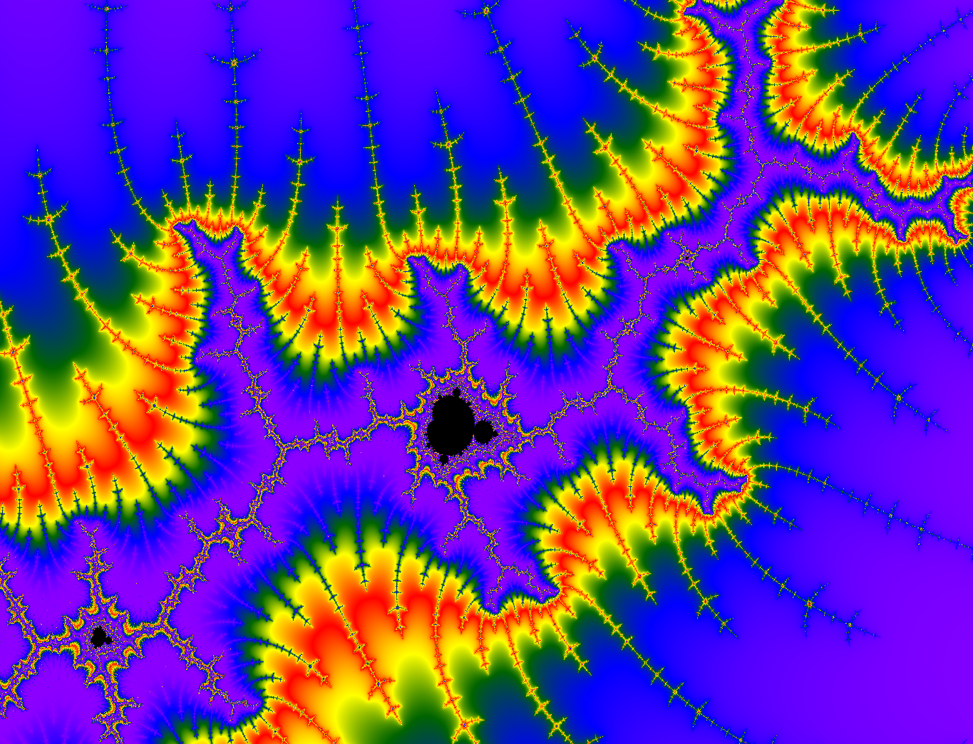
Today I added a couple of features to Marzipan, my fractal generator, so I’m going to show a few images of what I worked on 🙂
First, I refactored the orbit trap coloring to be able to expand it with other types of orbit traps; then I added the implementation for line orbit traps. Turns out, adding random line and point orbit traps is pretty fun, and can yield pretty results!
A mix of line and point trap orbits
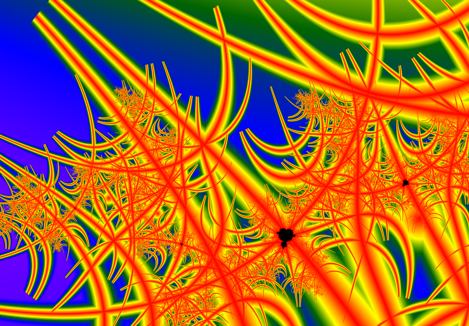
The other thing that I did was to add “multi-color palettes”: instead of giving a “beginning color” and an “end-color”, I can now pass a set of colors that will get used over the value interval. Which means, I can get much more colorful (and hence incredibly more eye-hurting) images!
Yay, rainbows!
And, well, I can also combine these two approaches to get NEON RAINBOWS!
Yay, NEON RAINBOWS!
Finally, I also played a bit with the ratios of the image that I generate – the goal is to not distort the general shape of the bulbs when zooming in the image. This is still pretty unsatisfactory, I need to make that work better (and to understand exactly how the size of the Qt window interacts with my window manager, because I’m probably making my life more complicated than it strictly needs to be there).
I had a lot of fun today implementing all of that, and then losing myself into finding fun colorings and fun trap orbits and all that kind of things. Now, the issue is that if I have more colors, I have more leeway to generate REALLY UGLY IMAGES, and I may need to develop a bit of taste if I want to continue doing pretty stuff 😉
Now what crossed my mind today:
I believe I have a bug, either in the multi-color palette or in the orbit trap coloring – I’ve seen suspicious things when zooming on certain parts (colors changing whereas they should not have), so I’ll need to track it and fix it. I also made performance worse when playing with multiple orbits for laziness reasons, I’ll need to fix that too.
I have some more things that I want to experiment with on orbit traps – I think there’s some prettiness I haven’t explored yet and I want to do that.
I should really start thinking about getting a better UI. I want a have better UI, I don’t want to code the better UI 😛
I should at least add a proper way to save an image instead of relying on getting them from the place where I dump them before displaying them – that would be helpful.
I should also find a way to import/export “settings” so that a given image can be reproduced – right now it’s very ephemeral. Which is not necessarily a bad thing 😉
I can probably improve the performance of the “increasing the number of iterations” operation, and I should do that.
The “image ratio” thing is still very fuzzy and I need to think a bit more about what I want and how to do it.
About a year ago, I wrote a post called “The one with the meditation“. It’s on my French blog, because at that time I had written it in French first, and thought it was worth it to translate it in English there. I considered moving it here, but decided against it – instead, I’m going to write an update 🙂 And write it as Q&A again, because that worked reasonably well for the first post, even if it’s pretty contrived 🙂
So, you’re still meditating every day?
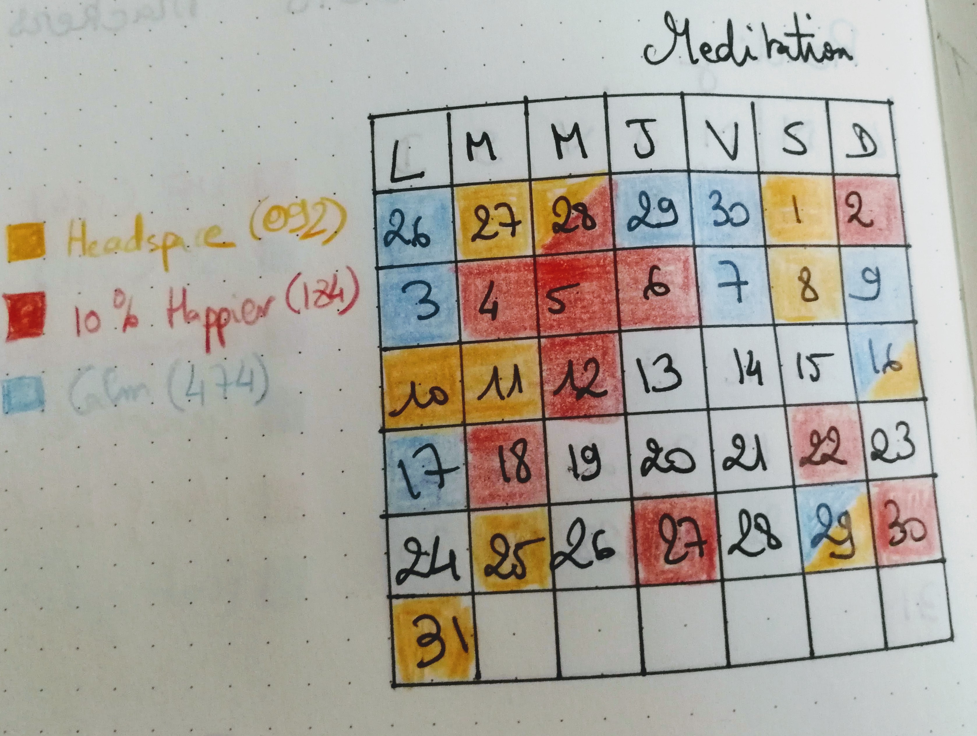
I’m going to say “yes, but there are days where I don’t”. My intent is to meditate every day. Sometimes I fail at it. I started journaling at the end of November, and I do have a “Meditation” tracker on it, and that’s what it looked like for “end of November / December”:
That’s probably the worst month that I’ve had in a while – but there have definitely been more lapses in the past few months than in the first six months of my practice.
All in all, I’d say it’s most definitely a part of my “self-care” routine. I haven’t been that diligent at self-care in the past few months; hence, some slippage. My new year’s resolution, by the way, is the umbrella “be better at self-care”, so maybe that will help 😉
Did your practice change in any way?
A bit. The general gist of it – sitting with a guided meditation – didn’t change much. But I’m now typically sitting cross-legged on the couch or the bed instead of sitting on a chair; and I changed my “guided meditation” habits a bit. I used to use only Headspace – I’ve been experimenting with other apps. That’s what the colors in the tracker above are: “what app did I use that day”. I gave a try to Calm: I don’t think it’s a fit for me right now, I find it too corny for my taste. I still like Headspace for the “straightforwardness” of it. I do like 10% Happier a lot because it’s more fun and there’s an instructor there (Jeff Warren) that I particularly like.
I also started training towards unguided meditation (with the Headspace Pro packs that do… just that), and that’s something I want to explore a bit more soon. In particular, I heard about Yet Another App, Insight Timer, that allows to define timers, including a few (or a lot of) intermediary sounds as a “safety net” on the whole “getting lost in thought” and/or “falling asleep” that may be helpful. We’ll see how that goes.
Also, while Headspace is pretty “focus-oriented”, there’s a bit more variety in 10% Happier, including along the topics of loving-kindness and compassion. Those are still very new to me. I used to reject the concept as “corny” and “not for me” and so on, but after a tiny bit of practice in that area, I find myself liking it way more than I thought I would, and to find the whole concept helpful as well.
Finally, there’s a meditation studio that opened almost literally next door to where I live; I’ve been trying to gather some courage to visit it, but so far the “fear of new stuff especially when it involves me being alone with a bunch of new people” has won.
Did your perspective about what it brings you change?
Not much. I still do enjoy the “getting a break from the chatter” part of it, and the brief moment of quiet that I usually (but not always) get. I also do think that when Brain is Acting Up – getting into an anxiety attack, or a self-hate spiral, or that sort of unpleasant things – I now generally have a tiiiiiny bit of distance from it, in that I see what is happening, and there is now a tiny place in my head that’s reassuring me that yup, the spiral sucks, but it will eventually be over. That seems to helps me getting out of that kind of states slightly faster – and, more importantly, to not chew on “the fact that this happened” for hours or days afterwards. (Not sure if that one is meditation-related, therapy-related, or a bit of both, but I’ll take it either way 🙂 )
The other main point is that I now do identify “meditation” as a large part of what I put into “self-care” – that also includes things like getting enough sleep, exercising, getting enough recovery time, and eating properly. And, like any other element in that category: the better I am at sticking to the routine that works, the better I feel – even if it’s sometimes super annoying that it’s necessary. So, in a way, it’s “it’s not that it brings me things that I can actually pinpoint, it’s more that if I stop doing it, Brain is usually Acting Up more”.
Any new resources to recommend?
I did mention two apps:
Calm – as I mentioned, I don’t think it works for me right now, but the app itself is well-made and has a fair amount of content. And there’s a lot of people who are happy with it, so you might be one of them as well.
Insight Timer – I have actually not used this one yet, but I’ve heard good things. They advertise that they have a lot more free content than the other meditation apps; I haven’t checked that statement but it seems plausible.
Book-wise, in the past year, I read two meditation-related books:
Full Catastrophe Living: Using the Wisdom of Your Body and Mind to Face Stress, Pain, and Illness, by Jon Kabat-Zinn. That one is a fairly heavy book about meditation and mindfulness. It’s essentially a “MBSR HowTo”, where MBSR stands for Mindfulness-Based Stress Reduction, a program developed by Kabat-Zinn that seems to be in large part used for people suffering from chronic pain. There was a lot of very interesting things and insights in this book (I do, in particular, remember about a part where he talks about the mechanics of breathing and the diaphragm and felt slightly mind-blown because I had never asked myself how it worked). At first, I was quite irritated by the amount of “Mr X. with this and that symptom came to a MBSR workshop and after 8 weeks was so much better”, but once I reframed my “okay, we get it, your thing is cool” into “let me give a lot of examples so that the reader has a chance to relate to one” it was better.
Altered Traits, by Daniel Goleman and Richard Davidson. Goleman and Davidson look at academic research on meditation, and it’s fascinating. Their interest is mostly about how long meditation practice (we’re talking tens of thousands of hours over a life time, compared to my paltry 90 hours over a couple of years) have an influence on the brain itself – what they called permanent “altered traits”, as opposed (by them) to the transient “altered states” than can sometimes be experienced during meditation. The book is a bit meandering and a bit self-serving at times, but I still found it very interesting.
In the previous episode, I explained two ways to sort books, and I counted the elementary operations I needed to do that, and I estimated the number of operations depending on the number of books that I wanted to sort. In particular, I looked into the best case, worst case and average case for the algorithms, depending on the initial ordering of the input. In this post, I’ll say a bit more about best/worst/average case, and then I’ll refine the notion of algorithmic complexity itself.
The “best case” is typically analyzed the least, because it rarely happens (thank you, Murphy’s Law.) It still gives bounds of what is achievable, and it gives a hint on whether it’s useful to modify the input to get the best case more often.
The “worst case” is the only one that gives guarantees. Saying that my algorithm, in the worst case, executes in a given amount of time, guarantees that it will never take longer – although it can be faster. That type of guarantees is sometimes necessary. In particular, it allows to answer the question of what happens if an “adversary” provides the input, in a way that will make the algorithm’s life as difficult as possible – a question that would interest cryptographers and security people for example. Having guarantees on the worst case means that the algorithm works as desired, even if an adversary tries to make its life as miserable as possible. The drawback of using the worst case analysis is that the “usual” execution time often gets overestimated, and sometimes gets overestimated by a lot.
Looking at the “average case” gives an idea of what happens “normally”. It also gives an idea about what happens if the algorithm is repeated several times on independent data, where both the worst case and the best case can happen. Moreover, there is sometimes ways to avoid the worst cases, so the average case would be more useful in that case. For example, if an adversary gives me the books in an order that makes my algorithm slow, I can compensate that by shuffling the books at the beginning so that the probability of being in a bad case is low (and does not depend on my adversary’s input). The drawback of using the average case analysis is that we lose the guarantee that we have on the worst case analysis.
For my book sorting algorithms, my conclusions were as follows:
For the first sorting algorithm, where I was searching at each step for a place to put the book by scanning all the books that I had inserted so far, I had, in the best case, operations, in the worst case, operations, and in the average case, . operations.
For the second sorting algorithm, where I was grouping book groups two by two, I had, in all cases, operations.
I’m going to draw a figure, because figures are pretty. If the colors are not that clear, the plotted functions and their captions are in the same order.
It turns out that, when talking about complexity, these formulas (, , , ) would not be the ones that I would use in general. If someone asked me about these complexities, I would answer, respectively, that the complexities are , (or “quadratic”), again, and .
This may seem very imprecise, and I’ll admit that the first time I saw this kind of approximations, I was quite irritated. (It was in physics class, so I may not have been in the best of moods either.) Since then, I find it quite handy, and even that it makes sense. The fact that “it makes sense” has a strong mathematical justification. For the people who want some precision, and who are not afraid of things like “limit when x tends to infinity of blah blah”, it’s explained there: http://en.wikipedia.org/wiki/Big_O_notation. It’s vastly above the level of the post I’m currently writing, but I still want to justify a couple of things; be warned that everything that follows is going to be highly non-rigorous.
The first question is what happens to smaller elements of the formulas. The idea is that only keep what “matters” when looking at how the number of operations increases with the number of elements to sort. For example, if I want to sort 750 books, with the “average” case of the first algorithm, I have . For 750 books, the two parts of the sum yield, respectively, 140625 and… 1687. If I want to sort 1000 books, I get 250000 and 2250. The first part of the sum is much larger, and it grows much quicker. If I need to know how much time I need, and I don’t need that much precision, I can pick and discard – already for 1000 books, it contributes less than 1% of the total number of operations.
The second question is more complicated: why do I consider as identical and , or and ? The short answer is that it allows to make running times comparable between several algorithms. To determine which algorithm is the most efficient, it’s nice to be able to compare how they perform. In particular, we look at the “asymptotic” comparison, that is to say what happens when the input of the algorithm contains a very large number of elements (for instance, if I have a lot of books to sort) – that’s where using the fastest algorithm is going to be at most worth it.
To reduce the time that it takes an algorithm to execute, I have two possibilities. Either I reduce the time that each operation takes, or I reduce the number of operations. Suppose that I have a computer that can execute one operation by second, and that I want to sort 100 elements. The first algorithm, which needs operations, finishes after 2500 seconds. The second algorithm, which needs operations, finishes after 1328 seconds. Now suppose that I have a much faster computer to execute the first algorithm. Instead of needing 1 second per operation, it’s 5 times faster, and can execute an operation in 0.2 seconds. That means that I can sort 100 elements in 500 seconds, which is faster than the second algorithm on the slower computer. Yay! Except that, first, if I run the second algorithm of the second computer, I can sort my elements five times faster too, in 265 seconds. Moreover, suppose now that I have 1000 elements to sort. With the first algorithm on the fast computer, I need seconds, and with the second algorithm on the much slower computer, seconds.
That’s the idea behind removing the “multiplying numbers” when estimating complexity. Given an algorithm with a complexity “” and algorithm with a complexity ““, I can put the first algorithm on the fastest computer I can: there will always be a number of elements for which the second algorithm, even on a very slow computer, will be faster than the first one. The number of elements in question can be very large if the difference of speed of the computers is large, but since large numbers are what I am interested in anyway, that’s not a problem.
So when I compare two algorithms, it’s much more interesting to see that one needs “something like ” operations and one needs “something like ” operations than to try to pinpoint the exact constant that multiplies the or the .
Of course, if two algorithms need “something along the lines of operations”, asking for the constant that is multiplying that is a valid question. In practice, it’s not done that often, because unless things are very simple and well-defined (and even then), it’s very hard to determine that constant exactly, depending on how you implement it with a programmation language. It would also require to ask exactly what an operation is. There are “classical” models that allow to define all these things, but linking them to current programming languages and computers is probably not realistic.
Everything that I talked about so far is function of , which is in general the “size of the input”, or the “amount of work that the algorithm has to do”. For books to sort, it would be the number of books. For graph operations, it would be the number of vertices of graphs, and/or the number of edges. Now, as “people who write algorithms”, given an input of size , what do we like, what makes us frown, what makes us run very fast in the other direction?
The “constant time algorithms” and “logarithmic time algorithms” (whose numbers of operations are, respectively, a constant that does not depend on or “something like “) are fairly rare, because with operations (or a constant number of operations), we don’t even have the time to look at the whole input. So when we find an algorithm of that type, we’re very, very happy. A typical example of a logarithmic time algorithm is searching an element in a sorted list. When the list is sorted, it is not necessary to read it completely to find the element that we’re looking for. We can start checking if it’s before or after the middle element, and search in the corresponding part of the list. Then we check if it’s before or after the middle of the new part of the list, and so on.
We’re also very happy when we find a “linear time algorithm” (the number of operations is “something like “). That means that we read the whole input, make a few operations per element of the input, and bam, done. is also usually considered as “acceptable”. It’s an important bound, because it is possible to prove that, in standard algorithmic models (which are quite close to counting “elementary” operations), it is not possible to sort elements faster than with operations in the general case (that is to say, without knowing anything about the elements or the order in which they are). There are a number of algorithms that require, at some point, some sorting: if it is not possible to get rid of the sorting, such an algorithm will also not get below operations.
We start grumbling a bit at , , and to grumble a lot on greater powers of . Algorithms that can run in operations, for some value of (even 1000000), are called “polynomial”. The idea is that, in the same way that a algorithm will eventually be more efficient than a algorithm, with a large enough input, a polynomial algorithm, whatever , will be more efficient than a -operation algorithm. Or than a -operation algorithm. Or even than a -operation algorithm.
In the real life, however, this type of reasoning does have its limits. When writing code, if there is a solution that takes 20 times (or even 2 times) less operations than another, it will generally be the one that we choose to implement. And the asymptotic behavior is only that: asymptotic. It may not apply for the size of the inputs that are processed by our code.
There is an example I like a lot, and I hope you’ll like it too. Consider the problem of multiplying matrices. (For people who never saw matrices: they’re essentially tables of numbers, and you can define how to multiply these tables of numbers. It’s a bit more complicated/complex than multiplying numbers one by one, but not that much more complicated.) (Says the girl who didn’t know how to multiply two matrices before her third year of engineering school, but that’s another story.)
The algorithm that we learn in school allows to multiply to matrices of size with operations. There exists an algorithm that is not too complicated (Strassen algorithm) that works in operations (which is better than ). And then there is a much more complicated algorithm (Coppersmith-Winograd and later) that works in operations. This is, I think, the only algorithm for which I heard SEVERAL theoreticians say “yeah, but really, the constant is ugly” – speaking of the number by which we multiply that to get the “real” number of operations. That constant is not very well-defined (for the reasons mentioned earlier) – we just know that it’s ugly. In practice, as far as I know, the matrix multiplication algorithm that is implemented in “fast” matrix multiplication librairies is Strassen’s or a variation of it, because the constant in the Coppersmith-Winograd algorithm is so huge that the matrices for which it would yield a benefit are too large to be used in practice.
And this funny anecdote concludes this post. I hope it was understandable – don’t hesitate to ask questions or make comments 🙂

 ,
,  or
or  . They’re kind of like the “unknowns” of an equation: we want to find values for
  means “or”, and
  means “and”. And the small bars above some of the letters indicate a negation. We combine these symbols with variables to get expressions, whose value can be computed as follow:
 , then
  , otherwise
  (
( is the opposite value of
  ; if
; if  , then
  and
and  , then
  . In other words,
  , otherwise
  . We read this: “


 :
:

 ,
,  are values that satisfy the formula).
 lines. For 5 variables,
  lines, that starts to be annoying to do by hand. For 20 variables,
  lines, the result is not necessarily instant anymore on a computer. And it continues growing: for
  variables, I need
  lines, which it grows faster and faster: the joys of power functions.
 . That’s a form where I have “groups” of variables linked by “
 . In that case, since within a group I need all the variables to be equal to 1 for the group to evaluate to 1, and since a variable and its negation cannot be equal both to 1, the group would evaluate to 0. So unless all the groups contain a variable and its negation, the formula is satisfiable – a fairly easy condition to verify.
 , we have “groups” of variables linked by


 . It so happens that, in classical computation models, we can’t do better than
  , where
  an arbitrary number (including very large numbers, as long as they do not depend on
  ,
,  ,
,  and
and  are called polynomial functions. Since I can sort elements in time
  , sorting is solved in polynomial time. It would also work if I could only sort elements in time
  , that would also be polynomial. The nice thing with polynomials is that they combine very well. If I make two polynomial operations, I’m still in polynomial time. If I make a polynomial number of polynomial operations, I’m still in polynomial time. The polynomial gets “bigger” (for instance, it goes from
  ), but it stays a polynomial.

 comparisons (maximum number of neighbors for a given vertex), we do at most
  operations, and the algorithm is polynomial. I don’t want to give much more details here because it’s not the main topic of my post, but if you want more details, ping me in the comments and I’ll try to explain better.


 operations, in the worst case,
  operations, and in the average case,
  . operations.
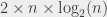 operations.
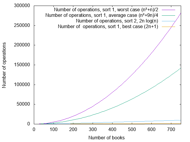
 . For 750 books, the two parts of the sum yield, respectively, 140625 and… 1687. If I want to sort 1000 books, I get 250000 and 2250. The first part of the sum is much larger, and it grows much quicker. If I need to know how much time I need, and I don’t need that much precision, I can pick
  and discard
  – already for 1000 books, it contributes less than 1% of the total number of operations.
 and
and  seconds, and with the second algorithm on the much slower computer,
  seconds.
 “) are fairly rare, because with
  , and to grumble a lot on greater powers of
  -operation algorithm. Or even than a
  -operation algorithm.
 with
with  operations (which is better than
  operations. This is, I think, the only algorithm for which I heard SEVERAL theoreticians say “yeah, but really, the constant is ugly” – speaking of the number by which we multiply that
.png)