maths – Balise's Blog

Proof by induction and proof by contradiction

Published on 19 April 201919 April 2019 by BaliseLeave a comment

This is the translation of an older post in French: Raisonnement par récurrence et raisonnement par l’absurde.

Let’s have a pretty short post so that I can refer to it later – I have another monster-post in the works, and I realized I needed the following elements to make it work, so here’s another post! I’m going to talk about two fundamental tools in the “proof toolbox”: the proof by induction and the proof by contradiction. These are tools that are explained in high school (well, they were in my French high school 20+ years ago 😉 ), and that you’ll see everywhere all the time, so let’s explain how it works.

Proof by induction

The idea of the induction proof is dominoes. Not the ones with the dots on them, the ones that you topple. You know that if you topple a domino, it falls. And if a domino falls, the next one falls as well. And you topple the first domino. Hence, all the dominoes fall.

Proofs by induction work in the same way. Suppose you have a property that depends on an natural number (positive integer), and you want to prove that it’s true for any natural number. First, you show that it’s true for a small natural number, say 0, 1 or 2 (sometimes the property doesn’t make much sense for 0 or 1). Then, you show that, if it’s true for a natural number $k$ , it’s also true for $k+1$ . So you have the “start” of the dominoes, the toppling (“it’s true for 0”), and the “chain” of dominoes (“if it’s true for $k$ , it’s true for $k+1$ “). If these two conditions are true, all the dominoes fall (“the property is true for all natural numbers greater than 0”).

Now this is where I’m a bit annoyed, because I have a an example that works, but the induction proof kind of sucks compared to another, which is much prettier. So I’m going to show both 😉

Suppose that I want to prove that the sum of all integers from 1 to $n$ (that is to say, $1 + 2 + 3 + 4 + ... + (n-2) + (n-1) + n$ ) equals $\displaystyle \frac{n(n+1)}{2}$ . I start with $n=1$ : $\displaystyle \frac{1(1+1)}{2} = \frac 2 2 = 1$ , so the base case is true.

Now, I suppose that it’s true for an arbitrary natural number $k$ that the sum of the integers from 1 to $k$ is equal to $\displaystyle \frac{k(k+1)}{2}$ , and I compute the sum of integers from 1 to $k+1$ : $1 + 2 + 3 + ... + (k-1) + k + (k+1)$ . This is equal to the sum of the integers from 1 to $k$ , plus $k+1$ . By induction hypothesis, this is equal to $\displaystyle \frac{k(k+1)}{2} + k+1 = \frac{k^2 + k + 2k + 2}{2} = \frac{k^2 + 3k + 2}{2}$ . For my proof to work out, I want the sum of integers from 1 to $k+1$ to be equal to $\displaystyle \frac{(k+1)(k+2)}{2}$ . And it so happens that $(k+1)(k+2)$ is precisely equal to $k^2 + 3k + 2$ .

So I have my base case, my induction step, and I proved exactly what I wanted to prove.

Now for the alternative, prettier proof. You consider a table with two lines and $n$ columns:

1  2   3   4  ... n-2 n-1 n
n n-1 n-2 n-3      3   2  1

and you compute the sum of all the numbers in the table. You can add up, for each column, both lines. Every column sums to $n+1$ : it’s the case for the first column, and at each step, you remove 1 from the first line, and you add 1 to the second line, so the sum stays the same (there’s actually a “hidden” induction proof in there!) There are $n$ columns, so if I add all these results, it sums to $n(n+1)$ . But if I group the sum in a different way, the first line is equal to the sum of integers from 1 to $n$ , the second line as well… so $n(n+1)$ is two times the sum of the integers from 1 to $n$ , which concludes the proof.

Proof by contradiction

Proofs by contradiction are sometimes dangerous, because they’re often misused or overused. I know some mathematicians who argue that a proof by contradiction is not very elegant, and that when one arises, it’s usually worth it to make the extra effort to try to turn it around in a non-contradiction proof. I still like the reasoning behind it, and it sometimes makes life much easier.

We want to prove that a proposition A is true. To prove A by contradiction, you make the hypothesis that A is false, you unroll a series of consequences that would be implied by the fact that A is false, and you arrive at something that you know is impossible. And if the fact that A is false implies an impossibility, it means that A is true, otherwise the universe collapses and it’s messy.

My favorite example is to prove that $\sqrt 2$ is irrational, that is to say that you can’t write it as $\displaystyle \frac p q$ where $p$ and $q$ are integers.

I need a tiny preliminary lemma: I’m claiming that if an integer $n$ is even, then its square $n^2$ is even, and that if $n^2$ is even, then $n$ is even. If $n$ is even, I can write $n = 2k$ (with $k$ integer). Then $n^2 = 4k^2 = 2 \times 2k^2$ , so $n^2$ is even. If $n$ is odd, I can write $n = 2k+1$ , so $n^2 = 4k^2 + 2k + 1 = 2(2k^2 + k) + 1$ , so $n^2$ is odd. So, if $n^2$ is even, then it can’t be that $n$ would be odd (because otherwise $n^2$ would be odd as well), so $n$ is even.

Now back to the irrationality of $\sqrt{2}$ . We make the hypothesis that we can write $\displaystyle \sqrt 2 = \frac p q$ . We can also make the assumption that the fraction is irreducible, because if it’s not, you can reduce it so that it is, so let’s assume that it’s the one we took from the beginning. (Note: a fraction $\displaystyle \frac p q$ is irreducible if there is no integer $k \geq 2$ such that $p$ and $q$ are both divisible by $k$ . If $k$ exists, we divide $p$ and $q$ by $k$ , and we get the fraction $\displaystyle \frac{p/k}{q/k}$ ).

So: I can write that $\sqrt 2 \times q = p$ . If I square this equality, I get $2q^2 = p^2$ . Since $q$ is an integer, $q^2$ is an integer, so $p^2$ is an even number (because it’s equal to twice an integer). But then, if $p^2$ is even, then $p$ is even as well, according to my preliminary lemma. So I can write $p = 2k$ and consequently $p^2 = 4k^2$ . But then, since $2q^2 = p^2 = 4k^2$ , I can also write $q^2 = 2k^2$ , so $q^2$ is even, so $q$ is even as well. But that’s not possible: $\displaystyle \frac p q$ is irreducible, so $p$ and $q$ cannot be both even! So something is wrong in my reasoning, and the only thing that can be wrong is my initial hypothesis, that is $\sqrt{2}$ is rational. Hence, $\sqrt{2}$ is irrational. Cute, isn’t it?

Planarity, minors and donuts

Published on 24 February 2019 by BaliseLeave a comment

Ce billet est la traduction d’un billet écrit initialement en français : TPA – Planarité, mineurs et donuts.

Let’s have a little bit of graph theory today – I want to present (without a proof) a fun result about graph planarity. Which means – first, let’s define a few things and draw a few pictures.

A graph is a set of vertices (“points”) connected by edges. To describe a graph, I can say “the set of vertices is labeled 1, 2, 3, 4 and 5, and I have edges between edges 1 and 2, 2 and 3, 3 and 4, 4 and 1, 1 and 3, 2 and 4, 1 and 5, and 4 and 5”. I can also draw it on a sheet of paper, and I can draw that statement in different ways: all the drawings here are drawings of the graph I just described.

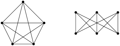
In these three drawings, two of them are plane: the graph is drawn such that edges of the graph do not cross. The first drawing is not plane: the edges 1-3 and 2-4 are crossing. A graph that can be drawn in the plane (that is to say, on a flat piece of paper) such that no two edges cross is called a planar graph. The fact that we have an adjective for such a graph should tell you that there exists non-planar graphs: graphs that cannot be drawn in the plane without crossing two edges. Two typical (and useful) examples are the complete graph on 5 vertices (5 vertices, and all possible edges) – denoted $K_5$ , and the complete bipartite graph on 3×2 vertices (2 groups $A$ and $B$ of three vertices, and all possible edges between vertices of group $A$ and vertices of group $B$ ), denoted $K_{3,3}$ . Here are their “usual” drawings; as we saw in the previous figure, these drawings are not unique. But you can search for a long long time for a drawing where no two edges cross (and not find it).

And there is a theorem (Wagner, 1937) that says that if a graph is not planar, it’s because somewhere in its structure it contains something that looks like $K_5$ or $K_{3,3}$ . More precisely:

A finite graph is planar if and only if it does not have $K_5$ or latex $K_{3,3}$ as a minor.

Okay, I cheated a bit, because I haven’t defined minor yet. So let’s do that:

A minor of a graph $G$ is a graph that is obtained from $G$ by doing any number of the following operations: removing an edge; removing a vertex; contracting a vertex.

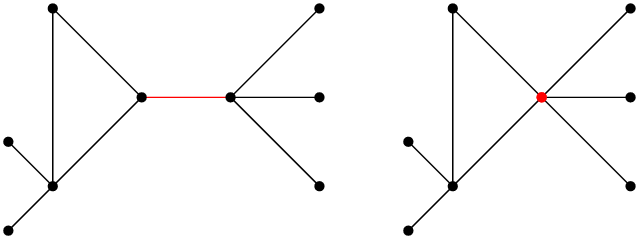
Removing an edge is easy: if two vertices are connected by an edge, we can decide that in fact they aren’t, and remove the edge. Removing a vertex is also easy: pick a vertex, remove it, and remove all the edges that are connected to it, because otherwise we don’t know where they’re going anyway. Contracting a vertex is a tiny bit more complicated: the idea is that we pick two vertices that are connected with an edge, and we “merge” them in a single vertex. The resulting vertex is connected to all the edges of the initial two vertices that were in the original graph. One can imagine “pinching” the two vertices that get closer and closer until BOOM they fuse together. For a small example, in which I contract the vertices connected by the red edge in a single vertex:

So what Wagner says is: “if I fiddle with a graph a bit and I manage to obtain $K_5$ or $K_{3,3}$ , then I cannot draw the graph without crossing edges. But if I cannot get $K_5$ or $K_{3,3}$ , then I can draw the graph without crossing.”

There’s a theorem that expands this idea of “forbidden minors”. It’s a theorem by Robertson and Seymour, and its proof spans over 20 papers, published from 1984 to 2003. The theorem is stated as follows:

Every family of graphs that is closed under minors can be defined by a finite set of forbidden minors.

Let’s explain. A family of graphs that is closed under minors is a set of graphs such that, if I take any graph in this family, and I take a minor of it (with the aforementioned definition), then the minor is also in that set of graphs. What Robertson and Seymour say is that, in such a family, there exists a finite set of forbidden minors: if a graph has a minor of that set, then that graph is not part of the family.

Wagner’s theorem is a restriction of Robertson-Seymour for planar graphs. Planar graphs are a family of graphs that is closed under minors: if I take a minor of a planar graph, I can still draw that minor without crossing any edge, so it is planar as well. And there is a finite set of forbidden minors, specifically $K_5$ or $K_{3,3}$ : if I find one of these minors in a graph, then the graph is not planar. Wagner, for the case of planar graphs, actually states the forbidden minors explicitly, which Robertson-Seymour does not.

And that’s the fun part: in general, we do not know the forbidden minors in question. We know they exist; we know there’s a finite number of them, but we do not know which they are. And, for a tiny example as a conclusion of this post: suppose now that I want to draw a graph not on a sheet of paper, but on a torus – or, if you want, on a donut.

Doughnuts! – https://coincuisine.pasithee.fr/2010/10/28/daring-bakers-doughnuts/

The idea would be to draw vertices on a donut, and to connect them with edges, exactly as I do in the plane. If I do that, and I can draw the graph without crossing edges, the graph is not planar anymore, but toroidal (or donutoidal if you want). The family of toroidal graphs is closed for minors, so there exists a set of forbidden minors for this family. So far, 17523 have been found. It is yet unknown how many there are in total. Fun, isn’t it?

(And if you want to find them all, you may want to start by making donuts.)

Intro to probability theory – part 2

Published on 14 February 2019 by Balise1 Comment

Ce billet a été traduit de sa version originale en français : Probabilités – Partie 2.

After the previous post about probability theory, here’s the second part, in which I’ll talk about random variables.

The idea of random variables is to have some way of dealing with events for which we do not exactly what happens (for instance, we roll a die), but still want to have some idea of what can happen. The die example is pretty simple, so using random variables may be a bit overkill, but let’s keep examples simple for now.

For a given experiment, we consider a variable, called $X$ , and look at all the values it can reach with the associated probability. If my experiment is “rolling a die and looking at its value”, I can define a random variable on the value of a 6-sided die and call it $X$ . For a full definition of $X$ , I need to provide all the possible values of $X$ (what we call the random variable’s domain) and their associated probabilities. For a 6-sided die, the values are the numbers from 1 to 6; for a non-loaded die, the probabilities are all equal to $\displaystyle \frac 1 6$ . We can write that as follows:

$\displaystyle \forall i \in \{1,2,3,4,5,6\}, \Pr[X = i] = \frac 1 6$

and read “for all $i$ in the set of values {1,2,3,4,5,6}, the probability that $X$ takes the value $i$ equals $\displaystyle \frac 1 6$ .

One of the basic ways to have an idea about the behaviour of a random variable is to look at its expectation. The expectation of a random variable can be seen as its average value, or as “suppose I roll my die 10000 times, and I average all the results (summing all the results and dividing by 10000), what result would I typically get?”

This expectation (written $E[X]$ ) can be computed with the following formula:

$E[X] = \displaystyle \sum_{i \in \text{dom}(X)} \Pr[x = i] \times i$

which can be read as “sum for all elements $i$ in the domain of $X$ of the probability that $X$ takes the value $i$ , times $i$ . In the die example, since the domain is all the integer numbers from 1 to 6, I can write

$\displaystyle \sum_{i=1}^6 \Pr[X = i] \times i$

which I can in turn expand as follows:

$\begin{aligned}E[X] &=& 1 \times \Pr[X = 1] + 2 \times \Pr[X = 2] + 3 \times \Pr[X = 3] \\ &+& 4 \times \Pr[X = 4] + 5 \times \Pr[X = 5] + 6 \times \Pr[X = 6]\end{aligned}$

Since, for my die, all the probabilities are equal to $\displaystyle \frac 1 6$ , I can conclude with

$\displaystyle E[X] = \frac 1 6 \times (1 + 2+3+4+5+6) = \frac{21}{6} = 3.5$

So the average value of a die over a large number of experiments is 3.5, as most tabletop gamers would know 😉

Now let’s look at a slightly more complicated example. Suppose that I have $n$ dice, and that I want to know how many 6s I can expect in my $n$ dice. From a handwavy point of view, we know that we will not get an exact answer for every time we roll $n$ dice, but that we can get a rough answer. There’s no reason there should be more or less 6s than 1s, 2s, 3s, 4s or 5s, so generally speaking the dice should be distributed approximately equally in the 6 numbers, so there should be approximately $\displaystyle \frac n 6$ 6s over $n$ dice. (The exception to that being me playing Orks in Warhammer 40k, in which case the expected number is approximately 3 6s over 140 dice.) Let us prove that intuition properly.

I define $Y$ as the random variable representing the number of 6s over $n$ dice. The domain of $Y$ is all the numbers from 0 to $n$ . It’s possible to compute the probability to have, for example, exactly 3 6s over $n$ dice, and even to get a general formula for $k$ dice, but I’m way too lazy to compute all that and sum over $n$ and so on. So let’s be clever.

There’s a very neat trick called linearity of expectation that says that the expectation of the sum of several random variables is equal to the sum of the expectations of said random variables, which we write

$E[A + B] = E[A] + E[B]$

This is true for all random variables $A$ and $B$ . Beware, though: it’s only true in general for the addition. We cannot say in general that $E[A \times B] = E[A] \times E[B]$ : that’s in particular true if the variables are independent, but it’s not true in general.

Now we’re going to define $n$ variables, called $Y_1, Y_2, ..., Y_n$ so that $Y$ is the sum of all these variables. We can define, for each variable $Y_1$ , the domain {0,1}, and we say that $Y_1$ is equal to 1 if and only if the die number 1 shows a 6. The other variables $Y_i$ are defined similarly, one for each die. Since I have $n$ variables, which take value 1 when their associated die shows a 6, I can write

$\displaystyle Y = \sum_{i = 1}^n Y_i$

This is where I use linearity of expectation:

$\displaystyle E[Y] = E\left[\sum_{i=1}^n Y_i\right] = \sum_{i=1}^n E[Y_i]$

The main trick here is that variables $Y_i$ are much simpler to deal with than $Y$ . With probability $\displaystyle \frac 1 6$ , they take value 1; with probability $\displaystyle \frac 5 6$ , they take value 0. Consequently, the expectation of $Y_i$ is also much easier to compute:

$\displaystyle E[Y_i] = 1 \times \frac 1 6 + 0 \times \frac 5 6 = \frac 1 6$

Plugging that in the previous result, we get the expectation of $Y$ :

$\displaystyle E[Y] = E\left[\sum_{i=1}^n Y_i\right] = \sum_{i=1}^n E[Y_i] = \sum_{i=1}^n \frac 1 6 = \frac n 6$

which is the result we expected.

Now my examples are pretty simple. But we can use that kind of tools in much more complicated situations. And there’s a fair amount of other tools that allow to estimate things around random variables, and to have a fairly good idea of what’s happening… even if we involve dice in the process.

Intro to probability theory – part 1

Published on 10 February 201910 February 2019 by Balise2 Comments

Ce billet est la traduction d’un billet écrit en français ici : Probabilités – partie 1

I’m eventually going to talk a bit about random algorithms, but before I do that, I need to talk about probability theory so that everyone is speaking the same language.

Probability theory is a bit annoying, because probability is something that many people use fairly often in their daily life, but it can be awfully counter-intuitive. That, or human beings suck at probability theory – also a possibility.

I kind of don’t want to formally define probability (“given a universe $\Omega$ , events”, blah blah blah… yeah, no, don’t want to do that), I’m going to try to explain things in a handwavy way, and hope for the best.

First, let me assume that everything I’m talking about here – unless mentioned otherwise explicitly – has “usual” properties: dice are not loaded, coins are real coins, etc.

Let us start with a classical example. If I flip a coin, what is the probability that it shows heads when it lands? The answer is 1/2: I have two possible events (the coin can show heads or tails), and they both have the same probability of occurring. Same thing if I roll a 6-sided die: the probability that it shows 4 is 1/6; I have six possible events that all have the same probability of occurring. In general, I’ll say that if I do an experiment (flipping a coin, rolling a die) that has $k$ possible outcomes, and that all of these outcomes have the same probability (“chance of happening”), then the probability of each of these outcomes (“events”) is $\displaystyle \frac 1 k$ .

It can happen that all the possible outcomes don’t have the same probability, but there are a few non-negotiable rules. A probability is always a number between 0 and 1. An event that never occurs has probability 0; an event that always occurs has probability 1. If I find a coin with two “heads” sides, and I flip it, it shows “heads” with probability 1 and “tails” with probability 0. Moreover, the sum of all the probabilities of all the possible outcomes of a given experience sums to 1. If I have $k$ events that have the same probability, we indeed have $\displaystyle k \times \frac 1 k = 1$ . If I have a die with three sides 1, two sides 2 and one side 3, the probability that it shows 1 is $\displaystyle \frac 3 6$ , the probability that it shows 2 is $\displaystyle \frac 2 6$ , and the probability that it shows 3 is $\displaystyle \frac 1 6$ ; the sum of all these is $\displaystyle \frac 3 6 + \frac 2 6 + \frac 1 6 = 1$ .

Now it gets a bit trickier. What is the probability that a (regular) 6-sided die shows 3 or 5? Well, the probability that it shows 3 is $\displaystyle \frac 1 6$ ; the probability that it shows 5 is $\displaystyle \frac 1 6$ , and the probability that it shows 3 or 5 is $\displaystyle \frac 1 6 + \frac 1 6 = \frac 1 3$ . But summing the individual probabilities only works if the events are exclusive, that is to say they cannot both be true at the same time: if I rolled a 5, then I can’t have a 3, and vice-versa.

It does not work if two events can both occur at the same time (non-exclusively). For instance, consider that flip a coin and roll a die, and I look at the probability that the coin lands on tails or that the die lands on 6. Then I CANNOT say that it’s equal to the probability of the coin landing on tails – $\displaystyle \frac 1 2$ -, plus the probability that the die lands on 6 – $\displaystyle \frac 1 6$ – for a total of $\displaystyle \frac 2 3$ . A way to see that is to tweak the experiment a bit to see that it doesn’t work all the time. For example, the probability that the die lands on 1,2, 3 or 4 is $\displaystyle \frac 4 6 = \frac 2 3$ . The probability that the coin lands on tails is $\displaystyle \frac 1 2$ . And it’s not possible that the combined probability of these two events (the die lands on 1, 2, 3 or 4, or the coin lands on tails) is the sum of both probabilities, because that would yield $\displaystyle \frac 2 3 + \frac 1 2 = \frac 7 6$ , which is greater than 1. (And a probability is always less or equal to 1).

What is true, though, is that if I have events $A$ and $B$ , then

$\Pr(A \cup B) \leq \Pr(A) + \Pr(B)$

where $\Pr(A)$ is “probability that $A$ occurs”, $\Pr(B)$ is “probability that $B$ occurs” and $\Pr(A \cup B)$ is “probability that $A$ occurs or that $B$ occurs”. Or, in a full sentence: the probability of the union of two events (event $A$ occurs or event $B$ occurs) is always less than or equal to the sum of the probabilities of both events. You can extend this to more events: the probability of the union of several events is less than or equal to the sum of the probabilities of the individual events. It may not seem very deep a result, but in practice it’s used quite often under the name “union bound”. The union bound does not necessarily yield interesting results. For the case “the die lands on 1, 2, 3 or 4, or the coin lands on tails”, it yields a bound at $\displaystyle \frac 7 6$ … and we already had a better bound by the fact that the probability is always less than 1. It is slightly more useful to bound the probability that the die lands on a 6 or that the coin lands on tails: we know that the probability is less than $\displaystyle \frac 2 3$ . When analyzing random algorithms, the union bound is often pretty useful, because the probabilities that we consider are often pretty small, and we can add a lot of them before the bound stops making sense. The union bound is often not enough to make a useful conclusion, but it’s very often a useful tool as a step of a proof.

For the example that I’ve been using so far, the best tool (because it gives an exact result) is the inclusion-exclusion principle. For two events $A$ and $B$ , it’s stated as follows:

$\Pr(A \cup B) = \Pr(A) + \Pr(B) - \Pr(A \cap B)$

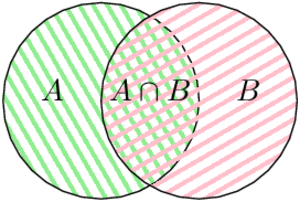
with the same notation as previously, and $\Pr(A \cap B)$ representing the probability that both events $A$ and $B$ occur. In a sentence: the probability that $A$ or $B$ occur is equals to the sum of the probabilities that either of them occurs, minus the probability that both $A$ and $B$ occur at the same time. The idea is that, if two events can occur at the same time, that probability is counted twice when summing the probabilities. It may be clearer with a small drawing (also known as Venn diagram):

If I count everything that is in the green area (corresponding to event $A$ ), and everything that is in the pink area (corresponding to event $B$ ), I count twice what is both in the green and pink area; if I want to have the correct result, I need to remove once what is common to both areas.

Now the question becomes – how to compute the probability of two events arriving at the same time? There’s the easy case, and the not so easy case. In the easy case, the events are independent: the probability that one occurs has no impact on the probability that the other one occurs. It’s is true (although not necessarily intuitive) if one is working with dice and coins and considering their individual results, but it’s a notion that requires a lot of care to apply (it’s not true anymore if I’m interested in the individual results and the sum of two dice, for example). Proving that two events are independent can be pretty complicated, and handling computations when they are not… as well.

When two events are independent, we have:

$\Pr(A \cap B) = \Pr(A) \times \Pr(B)$

that is to say that the probability that both events occur is equal to the product of the probabilities of both events. If I’m flipping a coin and rolling a die, the coin landing on tails has no impact on the die landing on 6. Both events are independent; the probability that both events occur is consequently $\displaystyle \frac 1 2 \times \frac 1 6 = \frac{1}{12}$ . Observe that this probability is smaller than $\displaystyle \frac 1 2$ and smaller than $\displaystyle \frac 1 6$ . It’s “obvious” since a probability is smaller than one, and that consequently multiplying two probabilities together yields a result that is smaller than both. Another way to see that is the fact that the probability that two independent event occur at the same time is less probable than the probability than only one of them occurs.

An example of two events that are not independent would be event $A$ “the die lands on 1” and event $B$ “the die lands on an odd number”. In that case, the events are not independent: if the die lands on 1, then it landed on an odd number; if the die lands on 2, it cannot land on an odd number as well. In that specific case, event $A$ is included in event $B$ , so it’s easy: the probability that both events occur is equal to the probability of the included event: $A \cap B$ is the same thing as $A$ . For a subtler example, one can define $A$ as “the die lands on 1, 4 or 6” and keep $B$ as “the die lands on an odd number”. These events are not independent either. The probability of $A$ and $B$ both occurring is $\displaystyle \frac 1 6$ , corresponding to the die landing on 1 (it’s the only case that’s both in 1, 4, 6 and odd). Multiplying the probabilities of A – $\displaystyle \frac 1 2$ – and B – $\displaystyle \frac 1 2$ – without paying attention yields $\displaystyle \frac 1 4$ and that’s how we get a mistake in our proof.

Last one for the road: I still want to talk about conditional probabilities. Conditional probabilities are a way to handle dependencies between events. We write $\Pr(A \mid B)$ , say “probability of $A$ given $B$ “, and understand “probability of $A$ knowing that $B$ occurs”. If $A$ and $B$ are independent, then $\Pr(A \mid B) = \Pr(A)$ : the fact that $B$ occurs does not have any impact on the occurrence of $A$ . For the previous case, where $A$ is the event “the die lands on 1” and $B$ is the event “the die lands on an odd number”, we can see the “given $B$ ” clause as a restriction of the possible events. The die landed on an odd number, it is known – so now, we know that it has the same probability to have landed on 1, 3 or 5, but a probability of 0 to have landed on 2, 4 or 6. Consequently, we have $\displaystyle \Pr(A \mid B) = \frac 1 3$ .

There’s a general formula for conditional probabilities:

$\displaystyle \Pr(A \mid B) = \frac{\Pr(A \cap B)}{\Pr(B)}$

It’s possible to show, from this formula, the fact that if A and B are independent, then $\Pr(A \mid B) = \Pr(A)$ , because then:

$\displaystyle \Pr(A \mid B) = \frac{\Pr(A) \times \Pr(B)}{\Pr(B)} = \Pr(A)$

That formula is also pretty useful in the other direction:

$\displaystyle \Pr(A \cap B) = \Pr(A \mid B) \times \Pr(B) = \Pr(B \mid A) \times \Pr(A)$

because it’s sometimes easier to understand what happens in the context of conditional probabilities than in the context of two non-independent events occurring.

In the next blog post, we’ll talk about random variables 🙂

NP-complete problems

Published on 21 January 2019 by BaliseLeave a comment

In a previous post, I tried to explain the P vs NP problem. I gave a rough definition of the NP complexity class: NP is the class of the problems for which, for each “yes” instance, I can get convinced in polynomial time that the answer is yes by providing me with a proof that it is indeed the case. And, at the end of that post, I vaguely mentioned (without naming it) the notion of NP-complete problems.

The usual definition of a NP-complete problem is that it’s a problem which belongs to NP, and which is NP-hard. So now I need to explain what NP-hard means. Informally, it’s a problem that is at least as hard as all other problems of the NP class. Another informal way to say that is that it’s at least as hard as another NP-hard problem. The problem with that definition is the bootstrap problem: you’d need a first NP-hard problem to compare it to the others.

The archetypal NP-hard problem is SAT, which was the topic of my previous post. Since SAT is also in NP, SAT is also the archetypal NP-complete problem. It’s not a priori obvious that SAT is NP-hard. But one can prove that even 3-SAT is NP-hard, where 3-SAT represents the CNF instances of SAT where all clauses have exactly 3 literals. I’m not going to go through the proof, because that would imply that I’d explain a lot of things that I kind of don’t want to explain. For the people who are interested in the topic, it’s been proven in 1971, and it is known as the Cook-Levin theorem.

Now that we do have a NP-hard problem, we can find other ones by reduction. We reduce a NP-hard problem (for instance, 3-SAT), to another problem that we want to prove is NP-hard (call that problem A). To do that, we show that if we can solve A efficiently (that is to say, in polynomial time), then we can solve 3-SAT efficiently.

The idea of that kind of proof is to take an arbitrary instance of the NP-hard problem, and we transform it, in polynomial time, into an instance of A that allows to conclude on the original instance. Now suppose that we can solve problem A (that is to say, any instance of problem A) in polynomial time. Then we can take any instance of SAT, transform it into an instance of problem A, solve the instance of problem A, and get a conclusion. The transformation is done in polynomial time; the solving of A is in polynomial time; summing both yields again a polynomial, so we can solve any instance of SAT in polynomial time, so we can solve SAT in polynomial time. Easy.

NP-complete problems are, in a way, “complexity equivalent”: if we know how to solve one in polynomial time, then we can solve all of them in polynomial time as well, and we can solve all problems from NP in polynomial time (since NP-hard problems are at least as hard as any problem from NP). So, if we find a way to solve in polynomial time all the instances of any NP-complete problem… we proved that P = NP. And won a million dollars. And surprised a whole lot of people.

There is a large set of problems that are known to be NP-hard, or NP-complete if they are as well in NP. And there are people who look at… exotic problems, shall we say: let me give a few links for the people who are interested and may get a laugh out of it:

The Hardness of the Lemmings Game, or Oh no, more NP-Completeness Proofs – an article that explains that Lemmings is NP-complete
A Survey of NP-Complete Puzzles – a paper that gathers a fair amount of results of that type
Gaming is a hard job, but someone has to do it! – talking about video games, including Boulder Dash, Doom, and Lode Runner. And Puzzle Bobble.

After this fun interlude, I’m going to give an example of reduction, so that you see that kind of proof works. I’m going to prove that the CLIQUE problem is NP-hard. It’s pretty much the basic example that everybody gives when they’re teaching that kind of things, but there must be a reason (I guess: it’s fairly easy to explain, and the reduction is also fairly easy compared to some others). What I’m explaining here is largely coming from the CLRS, that is to say the Cormen, Leiserson, Rivest and Stein, that is to say Introduction to Algorithms – that’s the reference book for A LOT of algorithms classes. (And I have a copy at home and a copy at work – you never know.)

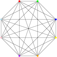
The CLIQUE problem is described as follows: given a graph (a set of vertices and edges) $G$ , does it contain a clique of size $k$ ? A clique of size $k$ is a set of $k$ vertices that are all connected to one another. For instance, this thing below is a clique of size 8. Also note that it does contain cliques of size 1 (single vertex), 2 (an edge), 3 (a triangle), 4, 5, 6, 7, since we can find sets of vertices of that size that are all connected to one another.

Let us reduce 3-SAT to that problem; since 3-SAT is NP-hard, CLIQUE will then be proven to be NP-hard as well. CLIQUE is in NP, because if I provide you with $k$ vertices, it’s possible to check that all these vertices are indeed connected to one another. So, if CLIQUE is NP-hard, CLIQUE is NP-complete.

To start with my reduction, I pick an arbitrary 3-SAT formula – more precisely, a 3-CNF-SAT formula (I explained the meaning of this in my post on SAT), which is a formula that has that look:

$(x_1 \vee x_2 \vee x_3) \wedge (\bar x_2 \vee x_4 \vee \bar x_5) \wedge (x_1 \vee \bar x_2 \vee \bar x_3) \wedge ...$

that is to say, a set of $m$ clauses connected by AND and composed of 3 literals connected by OR.

From there, we’re creating a graph that contains $3m$ vertices. Every vertex corresponds to a literal of the formula; vertices can be duplicated. For the above formula (truncated before the …), this yields the following vertices :

$x_1, x_2, x_3 ; \bar x_2, \bar x_4, \bar x_5 ; x_1, \bar x_2, \bar x_3$ .

Then, we add edges almost everywhere. We don’t add edges in the “groups” that correspond to the clauses, and we also do not add edges between literals that are not compatible, that is to say inverse of each other. If I have two literals $x_1$ and $\bar x_1$ , I’m not creating an edge between them. For the formula above, this is the graph in question:

And these are the edges that are NOT in the previous graph:

And now that we have that graph, we want to show that the SAT formula can be satisfied if and only if the graph (the first one) has a clique of size $m$ , where $m$ is the number of clauses in the SAT formula. So I need to prove two things:

if the formula can be satisfied, then the graph has a clique of size $m$ ,
if the graph has a clique of size $m$ , then the formula can be satisfied.

Let’s start with the first point. Suppose the formula can be satisfied. This means that we can assign a value to all the variables so that the formula is satisfied. This means that all clauses can be satisfied by this assignment. This also means that, for each clause, there’s a literal with value 1 (either a “positive” literal, for instance $x_1$ if the variable is assigned to 1, or a “negative” literal, for instance $\bar x_1$ , if the variable is assigned to 0). Now remember that we created vertices grouped by “clause”, so for each clause, we can pick the vertex corresponding to that 1-valued literal (and if several literals have value 1 in a clause, we can pick an arbitrary one). Since we pick a vertex by clause, and we have $m$ clauses, we have $m$ vertices. We now want to prove that these $m$ vertices form a clique, which means that there is an edge between every pair of vertices of that set. We constructed the graph such that there is no edge between two vertices of a given clause, and we’re fine there, because we chose exactly one vertex per clause. Moreover, there is no edge between a literal and its negation – we’re also fine there, because we only picked literals that have value 1, and $x_i$ and $\bar x_i$ can’t both have value 1. These are the only conditions for which there is no edge between two vertices; which means that our $m$ vertices are all connected with each other, which yields a clique of size $m$ , which is what we want.

Now, let’s look at the second point: if the graph has a clique of size $m$ , then the formula can be satisfied. Suppose that the graph has a clique of size $m$ . Since the vertices corresponding to the literals of a clause are not connected, this means that we have a vertex for each clause. We can give the value 1 to all the literals corresponding to these vertices. We cannot have a clique containing $x_i$ and $\bar x_i$ , because there would be no edge between these two vertices, which goes against the definition of a clique, where all edges are present. So if a clique of size $m$ exists, this means that we found, for each clause, a literal whose value can be 1, and that all of these literals are compatible with each other. And so, we can satisfy the formula corresponding to the graph, which we also wanted to prove.

So, if we can solve CLIQUE in polynomial time, then we can solve 3-SAT in polynomial time; since 3-SAT is NP-hard, CLIQUE is NP-hard, so CLIQUE is NP-complete, which concludes the proof.

Showing that a problem is NP-complete is, in a way, an indicator that the problem in question is difficult, but this needs to be mitigated a lot. For one thing, it does not say anything about a specific instance of the problem. It does not say anything about a specific subset of instances either – let me explain that. If I say that CLIQUE is difficult, it doesn’t mean that, for example, deciding whether a triangle (a clique of size 3) is in a graph is difficult. I can take all sets of 3 vertices, look at whether they form a triangle, and conclude. There are approximately $n^3$ sets of 3 vertices in a graph with $n$ vertices (okay, there’s exactly $\displaystyle \frac{n(n-1)(n-2)}{6}$ – anyway, roughly $n^3$ ), so I can actually decide that in polynomial time (because I’m doing $n^3$ operations which are basically checking if three edges are in a graph). So I can decide 3-CLIQUE in polynomial time. Well, I’m not going to be a millionaire with that, because the CLIQUE problem is wider than just 3. I can also decide 1000-CLIQUE (clique of size 1000) in polynomial time with the same principle. Well, it’s a polynomial of degree 1000, but who cares 😛

But, in the general case, I cannot decide whether a graph over $n$ vertices contains a clique of $\displaystyle \frac{n}{2}$ , or $\displaystyle \frac{n}{10000}$ vertices, or even $\log n$ vertices in polynomial time with this algorithm that looks at all groups of size $k$ (so, here, $k$ would be equal to $\displaystyle \frac{n}{2}$ , $\displaystyle \frac{n}{10000}$ , or $\log n$ ) and that looks at the edges of the group, because that would mean doing roughly $n^{n/2}$ , $n^{n/10000}$ and $n^{\log n}$ operations, respectively, and that in any case it’s not polynomial. And, generally speaking, nobody knows if it’s possible to do that in polynomial time, since CLIQUE is NP-complete and we don’t know if P is equal to NP. Many people think that not, but nobody knows.

Even that does not say anything about the difficulty of a specific instance. If I’m given a graph that contains $\displaystyle \frac{n(n-1)}{2}$ edges for $n$ vertices, then I can decide pretty easily that it does contain a clique of size $\displaystyle \frac{n}{2}$ , $\displaystyle \frac{n}{10000}$ and $\log n$ . That’s because a graph that has $\displaystyle \frac{n(n-1)}{2}$ for $n$ vertices contains all the possible edges for the graph: it’s a clique on $n$ vertices… which means that every subgraph over $k$ vertices, for all $k \leq n$ , is a clique of size $k$ . Same thing if I’m given a graph over $n$ vertices with 0 edge, it’s not going to be hard to say that it doesn’t contain a clique of size $\displaystyle \frac n 2$ .

SAT is also NP-hard, but can solve 2-CNF-SAT instances (where all clauses contain 2 literals) in polynomial, and even linear time. There are also SAT instances that are deemed “easy”, for instance the ones that have only few dependencies between the clauses: we know that we can to solve them, and we even know how (for the people who are interested in what I mean exactly by what I mean by “a few dependencies”, I’m thinking specifically about “the ones that are in the scope of the Lovász Local Lemma“, whose application to SAT is not trivial from the Wikipedia definition, but which might be clearer here).

Generally speaking, it may even be pretty difficult to create NP-hard instances of problems that we cannot solve in polynomial time. By the way, it’s not easy to show that we don’t know how to solve a given instance in polynomial time. We can find instances problem instances that are hard (i.e. require exponential time) for a given algorithm, and easy for another algorithm…

And that’s a bit of what happens in real life: we have instance of problems for which we know that the general case is NP-hard (or worse), and that we still solve without great difficulty. It can be that the problem is “small” (it’s not a huge problem to put an exponential algorithm on a problem of size 4), but it can also be that the problem belongs to an “easy” subset of instances. Considering that an instance of a problem is hard because the general problem is hard, and giving up on it (because we won’t know how to do it) may not be a good idea – it may be that we forgot to consider an easy restriction of the problem!

As usual, “it’s not that simple”. I’ve spent a fair amount of time with theory, and I tend to look at the problems themselves more than at given instances. But it’s sometimes nice to remember that stuff that’s “theoretically hard” can end up being “practically easy” – it’s a nice change from the things that are theoretically easy but that we don’t know how to do practically… 🙂

The SAT problem

Published on 19 January 201920 January 2019 by Balise1 Comment

Note: this is a translation with some re-writing of a previously published post: Le problème SAT.

I’m going to explain what the SAT problem is, because I’m going to talk about it a bit more soon. It’s one of the fundamental blocks around the P vs NP question; I’m going to write a blog post about NP-hard problems, but writing a post about SAT specifically is worth it. Also: I did my master thesis on SAT-related questions, so it’s a bit of a favorite topic of mine 🙂

SAT is a common abbreviation for “boolean satisfiability problem”. Everything revolves around the concept of boolean formulas, and a boolean formula can look like this:

$(x \vee y \vee z) \wedge (\bar x \vee \bar y) \wedge (\bar x \vee y \vee \bar z)$

Let me unpack this thing. The first concept is variables: here, $x$ , $y$ or $z$ . They’re kind of like the “unknowns” of an equation: we want to find values for $x$ , $y$ and $z$ . Moreover, we’re in a somewhat weird universe, the boolean universe: the only values $x$ , $y$ and $z$ can take are 0 or 1.

Then, we have some weird symbols. $\vee$ means “or”, and $\wedge$ means “and”. And the small bars above some of the letters indicate a negation. We combine these symbols with variables to get expressions, whose value can be computed as follow:

If $x = 1$ , then $\bar x = 0$ , otherwise $\bar x = 1$ ( $\bar x$ is the opposite value of $x$ ). We read this “not $x$ “.
If $x = 1$ , then $x \vee y = 1$ ; if $y = 1$ , then $x \vee y = 1$ ; if $x = 0$ and $y = 0$ , then $x \vee y = 0$ . In other words, $x \vee y = 1$ if $x = 1$ or $y = 1$ . Note that in this context, when we say “or”, we do not use exactly the same meaning than in everyday language: we mean “if $x = 1$ or if $y = 1$ or if both are equal to 1″. We read this: “ $x$ or $y$ “.
If $x = 1$ and $y = 1$ , then $x \wedge y = 1$ , otherwise $x \wedge y = 0$ . We read this: “ $x$ and $y$ “.

I’m summarizing all this in this table, for every possible value of $x$ and $y$ :

$\begin{array}{|c|c||c|c|c|c|} \hline x & y & \bar x &\bar y & x \vee y & x \wedge y \\ \hline 0 & 0 & 1 & 1 & 0 & 0 \\ \hline 0 & 1 & 1 & 0 & 1 & 0 \\ \hline 1 & 0 & 0 & 1 & 1 & 0 \\ \hline 1 & 1 & 0 & 0 & 1 & 1 \\ \hline \end{array}$

We can combine these expressions any way that we want to get boolean formulas. So the following examples are boolean formulas:

$x \wedge \bar y \wedge z \wedge t \wedge \bar u$
$(x \vee y) \wedge (\bar x \vee z) \wedge ((x \wedge z) \vee (z \wedge \bar t))$
$(x \vee y \vee z) \wedge (\bar x \vee \bar y) \wedge (\bar x \vee y \vee \bar z)$
$(x \wedge y \wedge z) \vee (\bar x \wedge \bar y) \vee (\bar x \wedge y \wedge \bar z)$

And then, by assigning values (0 or 1) to the individual variables, we can evaluate a formula for the assignment, that is to say, say if the value that the formula “computes” is 0 or 1. If the formula evaluates to 1 with an assignment, we say that this assignment satisfies the formula. And we say that a formula is satisfiable if there exists an assignment that makes it evaluate to 1 – hence the name of the problem, “boolean satisfiability”.

Boolean satisfiability in general is kind of “annoying” because it doesn’t have much structure to it: it’s hard to think about and it’s hard to say much about it, really. One thing that is always feasible, however, is to look at all the possibilities for all the variables, and see if there exists a combination of values that satisfies the formula. Picking one of the example above, and calling the formula $F$ :

$F = (x \vee y \vee z) \wedge (\bar x \vee \bar y) \wedge (\bar x \vee y \vee z)$

And let’s enumerate all possibilities:

$\begin{array}{|c|c|c||c|c|c||c|} \hline x & y & z & x \vee y \vee z & \bar x \vee \bar y & \bar x \vee y \vee z & F \\ \hline 0 & 0 & 0 & 0 & 1 & 1 & 0 \\ \hline 0 & 0 & 1 & 1 & 1 & 1 & 1 \\ \hline 0 & 1 & 0 & 1 & 1 & 1 & 1\\ \hline 0 & 1 & 1 & 1 & 1 & 1 & 1\\ \hline 1 & 0 & 0 & 1 & 1 & 0 & 0 \\ \hline 1 & 0 & 1 & 1 & 1 & 1 & 1 \\ \hline 1 & 1 & 0 & 1 & 0 & 1 & 0\\ \hline 1 & 1 & 1 & 1 & 0 & 1 & 0\\ \hline \end{array}$

This table answers the question “is there values of $x$ , $y$ and $z$ for which $F$ evaluates to 1 (the answer is yes) and it even goes further by giving said values (for instance, $x=1$ , $y = 0$ and $z = 1$ are values that satisfy the formula).

The issue is that it’s not really manageable to write such a table as soon as we get a lot of variables. The reason for that is that, for every variable, I need to check what happens for its 0 value and for its 1 value. So I have two choices for the first variable, two choices for the second variable, two choices for the third variable, and so on. The choices multiply with each other: similarly to the table above, I need a line for every possible combination of values of variables. For 3 variables, $2\times 2 \times 2 = 2^8 = 8$ lines. For 5 variables, $2 \times 2 \times 2 \times 2 \times 2 = 2^5 = 32$ lines, that starts to be annoying to do by hand. For 20 variables, $2^{20} = 1,048,576$ lines, the result is not necessarily instant anymore on a computer. And it continues growing: for $n$ variables, I need $2^n$ lines, which it grows faster and faster: the joys of power functions.

For the people who followed the previous explanations, this is NOT a polynomial time algorithm: it’s an exponential time algorithm. (Not even considering the fact that I’m only enumerating the possibilities and not evaluating the formula yet).

Since the general SAT problem seems fairly complicated to tackle, one can wonder if there are “subgroups” that are easy to solve, or that are easier to think about. And, indeed, there are such subgroups.

Suppose that, instead of getting an arbitrary combination of variables and symbols, I restrict myself of formulas such as this one: $(x \wedge y \wedge z) \vee (y \wedge \bar z \wedge t) \vee (u \wedge \bar y \wedge \bar t)$ . That’s a form where I have “groups” of variables linked by “ $\wedge$ “, themselves grouped by $\vee$ . Then that’s an “easy” case: for the formula to be satisfiable, I only need one of the “groups” to evaluate to 1 (because they are linked by “or” operators, so the formula evaluates to 1 if at least one of the groups evaluates to 1). And a given group evaluates to 1, unless it contains both one variable and its negation, like $x \wedge y \wedge \bar y$ . In that case, since within a group I need all the variables to be equal to 1 for the group to evaluate to 1, and since a variable and its negation cannot be equal both to 1, the group would evaluate to 0. So unless all the groups contain a variable and its negation, the formula is satisfiable – a fairly easy condition to verify.

If I consider the “opposite” of the previous setup, with formulas such as $(x \vee y \vee z) \wedge (\bar x \vee \bar y) \wedge (\bar x \vee y \vee z)$ , we have “groups” of variables linked by $\vee$ , themselves grouped by $\wedge$ . This type of formulas are called CNF formulas (where CNF means “conjunctive normal form”). A CNF formula is defined as a set of clauses (the “groups”), all linked by $\wedge$ symbols (“and”). A clause is a set of one or several literals that are linked by $\vee$ symbols (“or”). A literal is either a variable (for example $x$ ) or its negation (for example $\bar x$ ).

The question asked by an instance of the SAT problem is “can I find values for all variables such that the whole formula evaluates to 1?”. If we restrict ourselves to CNF formulas (and call the restricted problem CNF-SAT), this means that we want that all the clauses evaluate to 1, because since they are linked by “and” in the formula, I need that all of its clauses evaluate to 1. And for each clause to have value 1, I need at least one of the literals to have value 1 in the clause (I want the first literal or the second literal or the third literal or… to be equal to 1). As previously mentioned: it can happen that all the literals are equal to 1 – the clause will still be equal to 1.

It turns out that we can again look at subgroups within CNF formulas. Let us consider CNF formulas that have exactly 2 literals in all clauses – they are called 2-CNF formulas. The associated problem is called 2-CNF-SAT, or more often 2-SAT. Well, 2-SAT can be solved in linear time. This means that there exists an algorithm that, given any 2-CNF formula, can tell in linear time whether the formula is satisfiable or not.

Conversely, for CNF formulas that have clauses that have more than 2 literals… in general, we don’t know. We can even restrict ourselves to CNF formulas that have exactly 3 literals in each clause and still not know. The associated problem is called 3-CNF-SAT, or (much) more often 3-SAT.

From a “complexity class” point of view, 3-SAT is in NP. If I’m given a satisfiable 3-CNF formula and values for all variables of the formula, I can check in polynomial time that it works: I can check that a formula is satisfiable if I have a proof of it. (This statement is also true for general SAT formulas.)

What we do not know, however, is whether 3-SAT is in P: we do not know if there exists a polynomial time algorithm that allows us to decide if a 3-CNF formula can be satisfied or not in the general case. The difficulty of the problem still does not presume of the difficulty of individual instances. In general, we do not know how to solve the 3-SAT problem; in practice, 3-SAT instances are solved every day.

We also do not know whether 3-SAT is outside of P: we do not know if we need an algorithm that is “more powerful” than a polynomial time algorithm to solve the problem in the general case. To answer that question (and to prove it) would actually allow to solve the P vs NP problem – but to explain that, I need to explain NP-hard problems, and that’s something for the next post, in which I’ll also explain why it’s pretty reasonable to restrict oneself to 3-SAT (instead of the general SAT problem) when it comes to studying the theory of satisfiability 🙂

The “P vs NP” problem

Published on 16 January 201916 January 2019 by Balise1 Comment

Note: this is a translation of an older blog post written in French: Le problème « P est-il égal à NP ? ».

All right, I think I explained enough algorithmic complexity (part 1 and part 2) to start with a nice piece, which is to explain what is behind the “Is P equal to NP?” question – also called “P vs NP” problem.

The “P vs NP” problem is one of the most famous open problems, if not the most famous. It’s also part of the Millenium Prize problems, a series of 7 problems stated in 2000: anyone solving one of these problems gets awarded one million dollars. Only one of these problems has been solved, the Poincaré conjecture, proven by Grigori Perelman. He was awarded the Fields medal (roughly equivalent to a Nobel Prize in mathematics) for it, as well as the aforementioned million dollars; he declined both.

But enough history, let’s get into it. P and NP are called “complexity classes”. A complexity class is a set of problems that have common properties. We consider problems (for instance “can I go from point A to point B in my graph with 15 steps or less?”) and to put them in little boxes depending on their properties, in particularity their worst case time complexity (how much time do I need to solve them) and their worst case space complexity (how much memory do I need to solve them).

I explained in the algorithmic complexity blog posts what it meant for an algorithm to run in a given time. Saying that a problem can be/is solved in a given time means that we know how to solve it in that time, which means we have an algorithm that runs in that time and returns the correct solution. To go back to my previous examples, we saw that it was possible to sort a set of elements (books, or other elements) in time $n \log n$ . It so happens that, in classical computation models, we can’t do better than $n \log n$ . We say that the complexity of sorting is $n \log n$ , and we also say that we can sort elements in polynomial time.

A polynomial time algorithm is an algorithm that finishes with a number of steps that is less than $n^k$ , where $n$ is the size of the input and $k$ an arbitrary number (including very large numbers, as long as they do not depend on $n$ ). The name comes from the fact that functions such as $x \mapsto x$ , $x \mapsto x^2$ , $x \mapsto x^{10} + 15x^5$ and $x \mapsto x^k$ are called polynomial functions. Since I can sort elements in time $n \log n$ , which is smaller than $n^2$ , sorting is solved in polynomial time. It would also work if I could only sort elements in time $n^{419}$ , that would also be polynomial. The nice thing with polynomials is that they combine very well. If I make two polynomial operations, I’m still in polynomial time. If I make a polynomial number of polynomial operations, I’m still in polynomial time. The polynomial gets “bigger” (for instance, it goes from $n^2$ to $n^5$ ), but it stays a polynomial.

Now, I need to explain the difference between a problem and an instance of a problem – because I kind of need that level of precision 🙂 A problem regroups all the instances of a problem. If I say “I want to sort my bookshelf”, it’s an instance of the problem “I want to sort an arbitrary bookshelf”. If I’m looking at the length shortest path between two points on a given graph (for example a subway map), it’s an instance of the problem “length of shortest path in a graph”, where we consider all arbitrary graphs of arbitrary size. The problem is the “general concept”, the instance is a “concrete example of the general problem”.

The complexity class P contains all the “decision” problems that can be solved in polynomial time. A decision problem is a problem that can be answered by yes or no. It can seem like a huge restriction: in practice, there are sometimes way to massage the problem so that it can get in that category. Instead of asking for “the length of the shortest path” (asking for the value), I can ask if there is “a path of length less than X” and test that on various X values until I have an answer. If I can do that in a polynomial number of queries (and I can do that for the shortest path question), and if the decision problem can be solved in polynomial time, then the corresponding “value” problem can also be solved in polynomial time. As for an instance of that shortest path decision problem, it can be “considering the map of the Parisian subway, is there a path going from La Motte Piquet Grenelle to Belleville that goes through less than 20 stations?” (the answer is yes) or “in less than 10 stations?” (I think the answer is no).

Let me give another type of a decision problem: graph colorability. I like these kind of examples because I can make some drawings and they are quite easy to explain. Pick a graph, that is to say a bunch of points (vertices) connected by lines (edges). We want to color the vertices with a “proper coloring”: a coloring such that two vertices that are connected by a single edge do not have the same color. The graph colorability problems are problems such as “can I properly color this graph with 2, 3, 5, 12 colors?”. The “value” problem associated to the decision problem is to ask what is the minimum number of colors that I need to color the graph under these constraints.

Let’s go for a few examples – instances of the problem 🙂

A “triangle” graph (three vertices connected with three edges) cannot be colored with only two colors, I need three:

On the other hand, a “square-shaped” graph (four vertices connected as a square by four edges) can be colored with two colors only:

There are graphs with a very large number of vertices and edges that can be colored with only two colors, as long as they follow that type of structure:

And I can have graphs that require a very large number of colors (one per vertex!) if all the vertices are connected to one another, like this:

And this is where it becomes interesting. We know how to answer in polynomial time (where $n$ is of the number of vertices of the graph) to the question “Can this graph be colored with two colors?” for any graph. To decide that, I color an arbitrary vertex of the graph in blue. Then I color all of its neighbors in red – because since the first one is blue, all of its neighbors must be red, otherwise we violate the constraint that no two connected vertices can have the same color. We try to color all the neighbors of the red vertices in blue, and so on. If we manage to color all the vertices with this algorithm, the graph can be colored with two colors – since we just did it! Otherwise, it’s because a vertex has a neighbor that constrains it to be blue (because the neighbor is red) and a neighbor that constrains it to be red (because the neighbor is blue). It is not necessarily obvious to see that it means that the graph cannot be colored with two colors, but it’s actually the case.

I claim that this algorithm is running in polynomial time: why is that the case? The algorithm is, roughly, traversing all the vertices in a certain order and coloring them as it goes; the vertices are only visited once; before coloring a vertex, we check against all of its neighbors, which in the worst case all the other vertices. I hope you can convince yourself that, if we do at most $n$ (number of vertices we traverse) times $n-1$ comparisons (maximum number of neighbors for a given vertex), we do at most $n(n-1)$ operations, and the algorithm is polynomial. I don’t want to give much more details here because it’s not the main topic of my post, but if you want more details, ping me in the comments and I’ll try to explain better.

Now, for the question “Can this graph be colored with three colors?”, well… nobody has yet found a polynomial algorithm that allows us to answer the question for any instance of the problem, that is to say for any graph. And, for reasons I’ll explain in a future post, if you find a (correct!) algorithm that allows to answer that question in polynomial time, there’s a fair chance that you get famous, that you get some hate from the cryptography people, and that you win one million dollars. Interesting, isn’t it?

The other interesting thing is that, if I give you a graph that is already colored, and that I tell you “I colored this graph with three colors”, you can check, in polynomial time, that I’m not trying to scam you. You just look at all the edges one after the other and you check that both vertices of the edge are colored with different colors, and you check that there are only three colors on the graph. Easy. And polynomial.

That type of “easily checkable” problems is the NP complexity class. Without giving the formal definition, here’s the idea: a decision problem is in the NP complexity class if, for all instances for which I can answer “yes”, there exists a “proof” that allows me to check that “yes” in polynomial time. This “proof” allows me to answer “I bet you can’t!” by “well, see, I can color that way, it works, that proves that I can do that with three colors” – that is, if the graph is indeed colorable with 3 colors. Note here that I’m not saying anything about how to get that proof – just that if I have it, I can check that it is correct. I also do not say anything about what happens when the instance cannot be colored with three colors. One of the reasons is that it’s often more difficult to prove that something is impossible than to prove that it is possible. I can prove that something is possible by doing it; if I can’t manage to do something, it only proves that I can’t do it (but maybe someone else could).

To summarize:

P is the set of decision problems for which I can answer “yes” or “no” in polynomial time for all instances
NP is the set of decision problems for which, for each “yes” instance, I can get convinced in polynomial time that it is indeed the case if someone provides me with a proof that it is the case.

The next remark is that problems that are in P are also in NP, because if I can answer myself “yes” or “no” in polynomial time, then I can get convinced in polynomial time that the answer is “yes” if it is the case (I just have to run the polynomial time algorithm that answers “yes” or “no”, and to check that it answers “yes”).

The (literally) one-million-dollar question is to know whether all the problems that are in NP are also in P. Informally, does “I can see easily (i.e. in polynomial time) that a problem has a ‘yes’ answer, if I’m provided with the proof” also mean that “I can easily solve that problem”? If that is the case, then all the problems of NP are in P, and since all the problems of P are already in NP, then the P and NP classes contain exactly the same problems, which means that P = NP. If it’s not the case, then there are problems of NP that are not in P, and so P ≠ NP.

The vast majority of maths people think that P ≠ NP, but nobody managed to prove that yet – and many people try.

It would be very, very, very surprising for all these people if someone proved that P = NP. It would probably have pretty big consequences, because that would mean that we have a chance to solve problems that we currently consider as “hard” in “acceptable” times. A fair amount of the current cryptographic operations is based on the fact, not that it is “impossible” to do some operations, but that it’s “hard” to do them, that is to say that we do not know a fast algorithm to do them. In the optimistic case, proving that P = NP would probably not break everything immediately (because it would probably be fairly difficult to apply and that would take time), but we may want to hurry finding a solution. There are a few crypto things that do not rely on the hypothesis that P ≠ NP, so all is not lost either 😉

And the last fun thing is that, to prove that P = NP, it is enough to find a polynomial time algorithm for one of the “NP-hard” problems – of which I’ll talk in a future post, because this one is starting to be quite long. The colorability with three colors is one of these NP-hard problems.

I personally find utterly fascinating that a problem which is so “easy” to get an idea about have such large implications when it comes to its resolution. And I hope that, after you read what I just wrote, you can at least understand, if not share, my fascination 🙂

Understanding maths

Published on 14 January 2019 by Balise1 Comment

Note: this post is a translation of an older post written in French: Compréhension mathématique. I wrote the original one when I was still in university, but it still rings true today – in many ways 🙂

After two heavyweight posts, Introduction to algorithmic complexity 1/2 and Introduction to algorithmic complexity 2/2, here’s a lighter and probably more “meta” post. Also probably more nonsense – it’s possible that, at the end of the article, you’ll either be convinced that I’m demanding a lot of myself, or that I’m completely ridiculous 🙂

I’m quite fascinated by the working of the human brain. Not by how it works – that, I don’t know much about – but by the fact that it works at all. The whole concept of being able to read and write, for instance, still amazes me. And I do spend a fair amount of time thinking about how I think, how to improve how I think, or how to optimize what I want to learn so that it matches my way of thinking. And in all of that thinking, I redefined for myself what I mean by “comprehension”.

My previous definition of comprehension

It often happens that I moan about the fact that I don’t understand things as fast as I used to; I’m wondering how much of that is the fact that I’m demanding more of myself. There was a time where my definition “understanding” was “what you’re saying looks logical, I can see the logical steps of what you’re doing at the blackboard, and I see roughly what you’re doing”. I also have some painful memories of episodes such as the following:

“Here, you should read this article.
− OK.
<a few hours later>
− There, done!
− Already?
− Well, yeah… I’m a fast reader…
− And you understood everything?
− Well… yeah…
− Including why <obscure but probably profound point of the article>?
<blank look, sigh and explanations> (not by me, the explanations).

I was utterly convinced to have understood, before it was proven to me that I missed a fair amount of things. Since then, I learnt a few things.

What I learnt about comprehension

The first thing I learnt, is that “vaguely understand” is not “comprehend”, or at least not at my (current) level of personal requirements. “Vaguely understanding” is the first step. It can also be the last step, if it’s on a topic for which I can/want to do with superficial knowledge. I probably gained a bit of modesty, and I probably say way more often that I only have a vague idea about some topics.

The second thing is that comprehension does take time. Today, I believe I need three to four reads of a research paper (on a topic I know) to have a “decent” comprehension of it. Below that, I have “a vague idea of what the paper means”.

The third thing, although it’s something I heard a lot at home, is that “repeating is at the core of good understanding”. It helps a lot to have at least been exposed to a notion before trying to really grasp it. The first exposure is a large hit in the face, the second one is slightly mellower, and at the third one you start to know where you are.

The fourth thing is that my brain seems to like it when I write stuff down. Let me sing an ode to blackboard and chalk. New technology gave us a lot of very fancy stuff, video-projectors, interactive whiteboards, and I’m even going to throw whiteboards and Vellada markers with it. I may seem reactionary, but I like nothing better than blackboard and chalk. (All right, the blackboard can be green.) It takes more time to write a proof on the blackboard than to run a Powerpoint with the proof on it (or Beamer slides, I’m not discriminating on my rejection of technology 😉 ) . So yeah, the class is longer, probably. But it gives time to follow. And it also gives time to take notes. Many of my classmates tell me they prefer to “listen than take notes” (especially since, for blackboard classes, there is usually an excellent set of typeset lecture notes). But writing helps me staying focused, and in the end to listen better. I also scribble a few more detailed points for things that may not be obvious when re-reading. Sometimes I leave jokes to future me – the other day, I found a “It’s a circle, ok?” next to a potato-shaped figure, it made me laugh a lot. Oh and, as for the fact that I also hate whiteboards: first, Velleda markers never work. Sometimes, there’s also a permanent marker hiding in the marker cup (and overwriting with an erasable marker to eventually erase it is a HUGE PAIN). And erasable marker is faster to erase than chalk. I learnt to enjoy the break that comes with “erasing the blackboard” – the usual method in the last classes I attended was to work in two passes, one with a wet thingy, and one with a scraper. I was very impressed the first time I saw that 😉 (yeah, I’m very impressionable) and, since then, I enjoy the minute or two that it takes to re-read what just happened. I like it. So, all in all: blackboard and chalk for the win.

How I apply those observations

With all of that, I learnt how to avoid the aforementioned cringy situations, and I got better at reading scientific papers. And takes more time than a couple of hours 😉

Generally, I first read it very fast to have an idea of the structure of the paper, what it says, how the main proof seems to work, and I try to see if there’s stuff that is going to annoy me. I have some ideas about what makes my life easier or not in a paper, and when it gets in the “not” territory, I grumble a bit, even though I suppose that these structures may not be the same for everyone. (There are also papers that are just a pain to read, to be honest). That “very fast” read is around half an hour to an hour for a ~10-page article.

The second read is “annotating”. I read in a little more detail, and I put questions everywhere. The questions are generally “why?” or “how?” on language structures such that “it follows that”, “obviously”, or “by applying What’s-his-name theorem”. It’s also pretty fast, because there is a lot of linguistic signals, and I’m still not trying to comprehend all the details, but to identify the ones that will probably require me to spend some time to comprehend them. I also take note of the points that “bother” me, that is to say the ones where I don’t feel comfortable. It’s a bit hard to explain, because it’s really a “gut feeling” that goes “mmmh, there, something’s not quite right. I don’t know what, but something’s not quite right”. And it’s literally a gut feeling! It may seem weird to link “comprehension” to “feelings”, but, as far as I’m concerned, I learnt, maybe paradoxically, to trust my feelings to evaluate my comprehension – or lack thereof.

The third read is the longer – that’s where I try to answer all the questions of the second read and to re-do the computations. And to convince myself that yeah, that IS a typo there, and not a mistake in my computation or reasoning. The fourth read and following are refinements of the third read for the questions that I couldn’t answer during the third one (but for which, maybe, things got clearer in the meantime).

I estimate that I have a decent understanding of a paper when I answered the very vast majority of the questions from the second read. (And I usually try to find someone more clever than me for the questions that are still open). Even there… I do know it’s not perfect.

The ultimate test is to prepare a presentation about the paper. Do as I say and not as I do – I typically do that by preparing projector slides. Because as a student/learner, I do prefer a blackboard class, but I also know that it’s a lot of work, and that doing a (good) blackboard presentation is very hard (and I’m not there yet). Once I have slides (which, usually, allow me to still find a few points that are not quite grasped yet), I try to present. And now we’re back to the “gut feeling”. If I stammer, if there are slides that make no sense, if the presentation is not smooth: there’s probably still stuff that requires some time.

When, finally, everything seems to be good, the feeling is a mix between relief and victory. I don’t know exactly what the comparison would be. Maybe the people who make domino shows. You spend an enormous amount of time placing your dominos next to one another, and I think that at the moment where the last one falls without the chain having been interrupted… that must be that kind of feeling.

Of course, I can’t do that with everything I read, it would take too much time. I don’t know if there’s a way to speed up the process, but I don’t think it’s possible, at least for me, in any significant way. I also need to let things “simmer”. And there’s a fair amount of strong hypotheses on the impact of sleep on learning and memory; I don’t know how much of that can be applied to my “math comprehension”, but I wouldn’t be surprised if the brain would take the opportunity of sleep to tidy and make the right connections.

Consequently, it’s sometimes quite frustrating to let things at a “partial comprehension” stage – whether it’s temporary or because of giving up – especially when you don’t know exactly what’s wrong. The “gut feeling” is there (and not only on the day before the exam 😉 ). Sometimes, I feel like giving up altogether – what’s the point of trying, and only half understanding things? But maybe “half” is better than “not at all”, when you know you still have half of the way to walk. And sometimes, when I get a bit more stubborn, everything just clicks. And that’s one of the best feelings of the world.

Introduction to algorithmic complexity – 2/2

Published on 12 January 2019 by Balise3 Comments

Note: this is the translation of a post that was originally published in French: Introduction à la complexité algorithmique – 2/2.

In the previous episode, I explained two ways to sort books, and I counted the elementary operations I needed to do that, and I estimated the number of operations depending on the number of books that I wanted to sort. In particular, I looked into the best case, worst case and average case for the algorithms, depending on the initial ordering of the input. In this post, I’ll say a bit more about best/worst/average case, and then I’ll refine the notion of algorithmic complexity itself.

The “best case” is typically analyzed the least, because it rarely happens (thank you, Murphy’s Law.) It still gives bounds of what is achievable, and it gives a hint on whether it’s useful to modify the input to get the best case more often.

The “worst case” is the only one that gives guarantees. Saying that my algorithm, in the worst case, executes in a given amount of time, guarantees that it will never take longer – although it can be faster. That type of guarantees is sometimes necessary. In particular, it allows to answer the question of what happens if an “adversary” provides the input, in a way that will make the algorithm’s life as difficult as possible – a question that would interest cryptographers and security people for example. Having guarantees on the worst case means that the algorithm works as desired, even if an adversary tries to make its life as miserable as possible. The drawback of using the worst case analysis is that the “usual” execution time often gets overestimated, and sometimes gets overestimated by a lot.

Looking at the “average case” gives an idea of what happens “normally”. It also gives an idea about what happens if the algorithm is repeated several times on independent data, where both the worst case and the best case can happen. Moreover, there is sometimes ways to avoid the worst cases, so the average case would be more useful in that case. For example, if an adversary gives me the books in an order that makes my algorithm slow, I can compensate that by shuffling the books at the beginning so that the probability of being in a bad case is low (and does not depend on my adversary’s input). The drawback of using the average case analysis is that we lose the guarantee that we have on the worst case analysis.

For my book sorting algorithms, my conclusions were as follows:

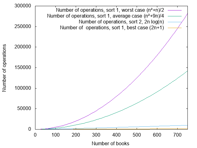
For the first sorting algorithm, where I was searching at each step for a place to put the book by scanning all the books that I had inserted so far, I had, in the best case, $2n-1$ operations, in the worst case, $\displaystyle \frac{n^2 + n}{2}$ operations, and in the average case, $\displaystyle \frac{n^2+9n}{4}$ . operations.
For the second sorting algorithm, where I was grouping book groups two by two, I had, in all cases, $2\times n \times\log_2(n)$ operations.

I’m going to draw a figure, because figures are pretty. If the colors are not that clear, the plotted functions and their captions are in the same order.

It turns out that, when talking about complexity, these formulas ( $2n-1$ , $\displaystyle \frac{n^2 + n}{2}$ , $\displaystyle \frac{n^2+9n}{4}$ , $2\times n \times\log_2(n)$ ) would not be the ones that I would use in general. If someone asked me about these complexities, I would answer, respectively, that the complexities are $n$ , $n^2$ (or “quadratic”), $n^2$ again, and $n \log n$ .

This may seem very imprecise, and I’ll admit that the first time I saw this kind of approximations, I was quite irritated. (It was in physics class, so I may not have been in the best of moods either.) Since then, I find it quite handy, and even that it makes sense. The fact that “it makes sense” has a strong mathematical justification. For the people who want some precision, and who are not afraid of things like “limit when x tends to infinity of blah blah”, it’s explained there: http://en.wikipedia.org/wiki/Big_O_notation. It’s vastly above the level of the post I’m currently writing, but I still want to justify a couple of things; be warned that everything that follows is going to be highly non-rigorous.

The first question is what happens to smaller elements of the formulas. The idea is that only keep what “matters” when looking at how the number of operations increases with the number of elements to sort. For example, if I want to sort 750 books, with the “average” case of the first algorithm, I have $\displaystyle \frac{n^2 + 9n}{4} = \displaystyle \frac{n^2}{4} + \frac{9n}{4}$ . For 750 books, the two parts of the sum yield, respectively, 140625 and… 1687. If I want to sort 1000 books, I get 250000 and 2250. The first part of the sum is much larger, and it grows much quicker. If I need to know how much time I need, and I don’t need that much precision, I can pick $\displaystyle \frac{n^2}{4}$ and discard $\displaystyle \frac{9n}{4}$ – already for 1000 books, it contributes less than 1% of the total number of operations.

The second question is more complicated: why do I consider as identical $n^2$ and $\displaystyle \frac{n^2}{4}$ , or $2n\log_2 n$ and $n \log n$ ? The short answer is that it allows to make running times comparable between several algorithms. To determine which algorithm is the most efficient, it’s nice to be able to compare how they perform. In particular, we look at the “asymptotic” comparison, that is to say what happens when the input of the algorithm contains a very large number of elements (for instance, if I have a lot of books to sort) – that’s where using the fastest algorithm is going to be at most worth it.

To reduce the time that it takes an algorithm to execute, I have two possibilities. Either I reduce the time that each operation takes, or I reduce the number of operations. Suppose that I have a computer that can execute one operation by second, and that I want to sort 100 elements. The first algorithm, which needs $\displaystyle \frac{n^2}{4}$ operations, finishes after 2500 seconds. The second algorithm, which needs $2n\log_2 n$ operations, finishes after 1328 seconds. Now suppose that I have a much faster computer to execute the first algorithm. Instead of needing 1 second per operation, it’s 5 times faster, and can execute an operation in 0.2 seconds. That means that I can sort 100 elements in 500 seconds, which is faster than the second algorithm on the slower computer. Yay! Except that, first, if I run the second algorithm of the second computer, I can sort my elements five times faster too, in 265 seconds. Moreover, suppose now that I have 1000 elements to sort. With the first algorithm on the fast computer, I need $0.2 \times \frac{1000^2}{4} = 50000$ seconds, and with the second algorithm on the much slower computer, $2 \times 1000 \times \log_2(1000) = 19931$ seconds.

That’s the idea behind removing the “multiplying numbers” when estimating complexity. Given an algorithm with a complexity “ $n^2$ ” and algorithm with a complexity “ $n \log n$ “, I can put the first algorithm on the fastest computer I can: there will always be a number of elements for which the second algorithm, even on a very slow computer, will be faster than the first one. The number of elements in question can be very large if the difference of speed of the computers is large, but since large numbers are what I am interested in anyway, that’s not a problem.

So when I compare two algorithms, it’s much more interesting to see that one needs “something like $n \log n$ ” operations and one needs “something like $n^2$ ” operations than to try to pinpoint the exact constant that multiplies the $n \log n$ or the $n^2$ .

Of course, if two algorithms need “something along the lines of $n^2$ operations”, asking for the constant that is multiplying that $n^2$ is a valid question. In practice, it’s not done that often, because unless things are very simple and well-defined (and even then), it’s very hard to determine that constant exactly, depending on how you implement it with a programmation language. It would also require to ask exactly what an operation is. There are “classical” models that allow to define all these things, but linking them to current programming languages and computers is probably not realistic.

Everything that I talked about so far is function of $n$ , which is in general the “size of the input”, or the “amount of work that the algorithm has to do”. For books to sort, it would be the number of books. For graph operations, it would be the number of vertices of graphs, and/or the number of edges. Now, as “people who write algorithms”, given an input of size $n$ , what do we like, what makes us frown, what makes us run very fast in the other direction?

The “constant time algorithms” and “logarithmic time algorithms” (whose numbers of operations are, respectively, a constant that does not depend on $n$ or “something like $\log n$ “) are fairly rare, because with $\log n$ operations (or a constant number of operations), we don’t even have the time to look at the whole input. So when we find an algorithm of that type, we’re very, very happy. A typical example of a logarithmic time algorithm is searching an element in a sorted list. When the list is sorted, it is not necessary to read it completely to find the element that we’re looking for. We can start checking if it’s before or after the middle element, and search in the corresponding part of the list. Then we check if it’s before or after the middle of the new part of the list, and so on.

We’re also very happy when we find a “linear time algorithm” (the number of operations is “something like $n$ “). That means that we read the whole input, make a few operations per element of the input, and bam, done. $n \log n$ is also usually considered as “acceptable”. It’s an important bound, because it is possible to prove that, in standard algorithmic models (which are quite close to counting “elementary” operations), it is not possible to sort $n$ elements faster than with $n \log n$ operations in the general case (that is to say, without knowing anything about the elements or the order in which they are). There are a number of algorithms that require, at some point, some sorting: if it is not possible to get rid of the sorting, such an algorithm will also not get below $n \log n$ operations.

We start grumbling a bit at $n^2$ , $n^3$ , and to grumble a lot on greater powers of $n$ . Algorithms that can run in $n^k$ operations, for some value of $k$ (even 1000000), are called “polynomial”. The idea is that, in the same way that a $n \log n$ algorithm will eventually be more efficient than a $n^2$ algorithm, with a large enough input, a polynomial algorithm, whatever $k$ , will be more efficient than a $2^n$ -operation algorithm. Or than a $1.308^n$ -operation algorithm. Or even than a $1.0001^n$ -operation algorithm.

In the real life, however, this type of reasoning does have its limits. When writing code, if there is a solution that takes 20 times (or even 2 times) less operations than another, it will generally be the one that we choose to implement. And the asymptotic behavior is only that: asymptotic. It may not apply for the size of the inputs that are processed by our code.

There is an example I like a lot, and I hope you’ll like it too. Consider the problem of multiplying matrices. (For people who never saw matrices: they’re essentially tables of numbers, and you can define how to multiply these tables of numbers. It’s a bit more complicated/complex than multiplying numbers one by one, but not that much more complicated.) (Says the girl who didn’t know how to multiply two matrices before her third year of engineering school, but that’s another story.)

The algorithm that we learn in school allows to multiply to matrices of size $n \times n$ with $n^3$ operations. There exists an algorithm that is not too complicated (Strassen algorithm) that works in $n^{2.807}$ operations (which is better than $n^3$ ). And then there is a much more complicated algorithm (Coppersmith-Winograd and later) that works in $n^{2.373}$ operations. This is, I think, the only algorithm for which I heard SEVERAL theoreticians say “yeah, but really, the constant is ugly” – speaking of the number by which we multiply that $n^{2.373}$ to get the “real” number of operations. That constant is not very well-defined (for the reasons mentioned earlier) – we just know that it’s ugly. In practice, as far as I know, the matrix multiplication algorithm that is implemented in “fast” matrix multiplication librairies is Strassen’s or a variation of it, because the constant in the Coppersmith-Winograd algorithm is so huge that the matrices for which it would yield a benefit are too large to be used in practice.

And this funny anecdote concludes this post. I hope it was understandable – don’t hesitate to ask questions or make comments 🙂

Mathematical intuition

Published on 9 January 20199 January 2019 by Balise1 Comment

Note: this post is a translation/adaptation of a post I wrote in French a few years ago: Intuition mathématique.

I initially wrote that post as a “warning” to my French-reading readers, saying “I might not manage to avoid annoying language tics such as ‘intuitively’, ‘obviously’, ‘it’s easy to see that'”. I think I got slightly better at that since then (or at least slightly better at noticing it and correcting it), but it’s still probably something I do.

I do try to avoid the “intuitive argument” when I explain something, because it used to make me quite anxious when I was on the receiving end of it and I had a hard time understanding why it was intuitive. But still, it does happen – it did happen in an exam once, to fail at explaining “why it’s intuitive”. Something that felt so brightly obvious that I had forgotten why it was so obvious. It’s quite annoying when someone points it out to you… especially when the “someone” is the examiner.

One of the most interesting articles I read on the topic was from Terry Tao, There’s more to mathematics than rigour and proofs. He distinguishes between three “stages” in math education:

the “pre-rigourous stage” – you make a lot of approximations, analogies, and probably you spend more time computing than theorizing
the “rigorous” stage – you try to do things properly, in a precise and formal way, and you work with abstract objects without necessarily having a deep understanding of what they mean (but you do work with them properly)
the “post-rigorous stage” – you know enough of your domain to know which approximations and which analogies are indeed valid, you have a good idea fairly quickly about what something is going to yield when the proof/computation is done, and you actually understand the concepts you work with.

Six years ago, when I wrote the original version of this post, I was considering myself a mix of the three. I did start to get some “intuition” (and I’ll explain later what I meant by that), but I was still pretty bad at finishing a complex computation properly. And, obviously, it did (and still does) depends on the domain: in “my” domain, I was approximately there; if you ask me right now to solve a differential equation or to work on complicated analysis, I’m probably going to feel very pre-rigourous. I’ve been out of university for a few years now, and there’s definitely some things that have regressed, that used to be post-rigourous and are now barely rigorous anymore (or that require a lot more effort to do things in a proper way, let’s say). One of the nice things that stayed, though, is that I believe I’m far less prone to make the confusion between “pre-rigourous” and “post-rigourous” than I used to be (which got me qualified as “sloppy” on more than one occasion).

Anyway, I believe that the categories are more fluid than what Tao says, but I also believe he’s right. And that there’s no need to panic when the person in front of you says: “it’s obvious/intuitive that”: she probably just has more experience than you do. And it’s sometimes hard to explain what became, with experience, obvious. If I say “it’s obvious than 2 + 3 = 5”, we’ll probably agree on it; if I ask “yeah, but why does 2 + 3 = 5 ?”, I’ll probably get an answer, but I may have some blank stares for a few seconds. It’s a bit of a caricature, but I think it’s roughly the idea.

In the everyday language, intuition is somewhat magical, a bit of “I don’t know why, but I believe that things are this way or that way, and that this or that is going to happen”. I tend to be very wary of intuition in everyday life, because I tend to be wary about what I don’t understand. In maths, the definition is roughly the same: “I think the result is going to look like that, and I feel that if I finish the proof it’s going to work”. The main advantage of mathematical intuition is that you can check it, understand why it’s correct or why it’s wrong. In my experience, (correct) intuition (or whatever you put behind that word) comes with practice, with having seen a lot of things, with the fact of linking things to one another. I believe that what people put behind “intuition” may be linking something new (a new problem) to something you’ve already seen, and to do this correctly. It’s also a matter of pattern matching. When it comes to algorithm complexity, which is the topic of the next two posts that I’ll translate, it’s “I believe this algorithm is going to take that amount of time, because it basically the same thing as this other super-well-known-thing that’s taking that amount of time”. The thing is, the associations are not always fully conscious – you may end up seeing the result first and explain it later.

It doesn’t mean that you can never be awfully wrong. Thinking that a problem is going to take a lot of time to solve (algorithmically speaking), when there is a condition that makes it much easier. Thinking that a problem is not very hard, and realizing it’s going to take way more time than ou thought. It still happens to me, in both directions. I believe that making mistakes is actually better than the previous step, which was “but how can you even have an idea on the topic?”

I don’t know how this intuition eventually develops. I know mine was much better after a few years at ETH than it was at the beginning of it. I also know it’s somewhat worse right now than when I just graduated. It’s still enough of a flux that I still get amazed by the fact that there are things now that are completely natural to me whereas they were a complete unknown a few years ago. Conversely, it’s sometimes pretty hard to realize that you once knew how to do things, and you forgot, by lack of practice (that’s a bit of my current state with my fractal generator).

But it’s also (still) new enough that I do remember the anxiety of not understanding how things can be intuitive for some people. So, I promise: I’m going to try to avoid saying things are intuitive or obvious. But I’d like you to tell me if I err in my ways, especially if it’s a problem for you. Also, there’s a fair chance that if I say “it’s intuitive”, it’s because I’m too lazy to get into explanations that seem obvious to me (but that may not be for everyone else). So, there: I’ll try to not be lazy 🙂

(Ironically: I did hesitate translating this blog post from French because it seemed like I was only saying completely obvious things in it and that it wasn’t very interesting. My guess is – it was less obvious to me 6 years ago when I wrote it, and so it’s probably not that obvious to people who spent less time than I did thinking about that sort of things 😉 )

	wiesmann on “What do I do with that…
	Balise on “What do I do with that…
	wiesmann on “What do I do with that…
	Scavenger Hunt #37… on Scavenger Hunt #32 –…
	wiesmann on 52Frames – 2022-49…