Ce billet est la traduction d’un billet écrit en français ici : Probabilités – partie 1

I’m eventually going to talk a bit about random algorithms, but before I do that, I need to talk about probability theory so that everyone is speaking the same language.

Probability theory is a bit annoying, because probability is something that many people use fairly often in their daily life, but it can be awfully counter-intuitive. That, or human beings suck at probability theory – also a possibility.

I kind of don’t want to formally define probability (“given a universe , events”, blah blah blah… yeah, no, don’t want to do that), I’m going to try to explain things in a handwavy way, and hope for the best.

First, let me assume that everything I’m talking about here – unless mentioned otherwise explicitly – has “usual” properties: dice are not loaded, coins are real coins, etc.

Let us start with a classical example. If I flip a coin, what is the probability that it shows heads when it lands? The answer is 1/2: I have two possible events (the coin can show heads or tails), and they both have the same probability of occurring. Same thing if I roll a 6-sided die: the probability that it shows 4 is 1/6; I have six possible events that all have the same probability of occurring. In general, I’ll say that if I do an experiment (flipping a coin, rolling a die) that has possible outcomes, and that all of these outcomes have the same probability (“chance of happening”), then the probability of each of these outcomes (“events”) is .

It can happen that all the possible outcomes don’t have the same probability, but there are a few non-negotiable rules. A probability is always a number between 0 and 1. An event that never occurs has probability 0; an event that always occurs has probability 1. If I find a coin with two “heads” sides, and I flip it, it shows “heads” with probability 1 and “tails” with probability 0. Moreover, the sum of all the probabilities of all the possible outcomes of a given experience sums to 1. If I have events that have the same probability, we indeed have . If I have a die with three sides 1, two sides 2 and one side 3, the probability that it shows 1 is , the probability that it shows 2 is , and the probability that it shows 3 is ; the sum of all these is .

Now it gets a bit trickier. What is the probability that a (regular) 6-sided die shows 3 or 5? Well, the probability that it shows 3 is ; the probability that it shows 5 is , and the probability that it shows 3 or 5 is . But summing the individual probabilities only works if the events are exclusive, that is to say they cannot both be true at the same time: if I rolled a 5, then I can’t have a 3, and vice-versa.

It does not work if two events can both occur at the same time (non-exclusively). For instance, consider that flip a coin and roll a die, and I look at the probability that the coin lands on tails or that the die lands on 6. Then I CANNOT say that it’s equal to the probability of the coin landing on tails – -, plus the probability that the die lands on 6 – – for a total of . A way to see that is to tweak the experiment a bit to see that it doesn’t work all the time. For example, the probability that the die lands on 1,2, 3 or 4 is . The probability that the coin lands on tails is . And it’s not possible that the combined probability of these two events (the die lands on 1, 2, 3 or 4, or the coin lands on tails) is the sum of both probabilities, because that would yield , which is greater than 1. (And a probability is always less or equal to 1).

What is true, though, is that if I have events and , then

where is “probability that occurs”, is “probability that occurs” and is “probability that occurs or that occurs”. Or, in a full sentence: the probability of the union of two events (event occurs or event occurs) is always less than or equal to the sum of the probabilities of both events. You can extend this to more events: the probability of the union of several events is less than or equal to the sum of the probabilities of the individual events. It may not seem very deep a result, but in practice it’s used quite often under the name “union bound”. The union bound does not necessarily yield interesting results. For the case “the die lands on 1, 2, 3 or 4, or the coin lands on tails”, it yields a bound at … and we already had a better bound by the fact that the probability is always less than 1. It is slightly more useful to bound the probability that the die lands on a 6 or that the coin lands on tails: we know that the probability is less than . When analyzing random algorithms, the union bound is often pretty useful, because the probabilities that we consider are often pretty small, and we can add a lot of them before the bound stops making sense. The union bound is often not enough to make a useful conclusion, but it’s very often a useful tool as a step of a proof.

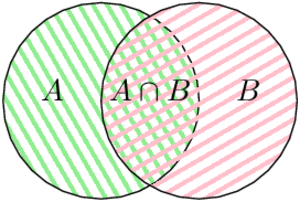
For the example that I’ve been using so far, the best tool (because it gives an exact result) is the inclusion-exclusion principle. For two events and , it’s stated as follows:

with the same notation as previously, and representing the probability that both events and occur. In a sentence: the probability that or occur is equals to the sum of the probabilities that either of them occurs, minus the probability that both and occur at the same time. The idea is that, if two events can occur at the same time, that probability is counted twice when summing the probabilities. It may be clearer with a small drawing (also known as Venn diagram):

If I count everything that is in the green area (corresponding to event ), and everything that is in the pink area (corresponding to event ), I count twice what is both in the green and pink area; if I want to have the correct result, I need to remove once what is common to both areas.

Now the question becomes – how to compute the probability of two events arriving at the same time? There’s the easy case, and the not so easy case. In the easy case, the events are independent: the probability that one occurs has no impact on the probability that the other one occurs. It’s is true (although not necessarily intuitive) if one is working with dice and coins and considering their individual results, but it’s a notion that requires a lot of care to apply (it’s not true anymore if I’m interested in the individual results and the sum of two dice, for example). Proving that two events are independent can be pretty complicated, and handling computations when they are not… as well.

When two events are independent, we have:

that is to say that the probability that both events occur is equal to the product of the probabilities of both events. If I’m flipping a coin and rolling a die, the coin landing on tails has no impact on the die landing on 6. Both events are independent; the probability that both events occur is consequently . Observe that this probability is smaller than and smaller than . It’s “obvious” since a probability is smaller than one, and that consequently multiplying two probabilities together yields a result that is smaller than both. Another way to see that is the fact that the probability that two independent event occur at the same time is less probable than the probability than only one of them occurs.

An example of two events that are not independent would be event “the die lands on 1” and event “the die lands on an odd number”. In that case, the events are not independent: if the die lands on 1, then it landed on an odd number; if the die lands on 2, it cannot land on an odd number as well. In that specific case, event is included in event , so it’s easy: the probability that both events occur is equal to the probability of the included event: is the same thing as . For a subtler example, one can define as “the die lands on 1, 4 or 6” and keep as “the die lands on an odd number”. These events are not independent either. The probability of and both occurring is , corresponding to the die landing on 1 (it’s the only case that’s both in 1, 4, 6 and odd). Multiplying the probabilities of A – – and B – – without paying attention yields and that’s how we get a mistake in our proof.

Last one for the road: I still want to talk about conditional probabilities. Conditional probabilities are a way to handle dependencies between events. We write , say “probability of given “, and understand “probability of knowing that occurs”. If and are independent, then : the fact that occurs does not have any impact on the occurrence of . For the previous case, where is the event “the die lands on 1” and is the event “the die lands on an odd number”, we can see the “given ” clause as a restriction of the possible events. The die landed on an odd number, it is known – so now, we know that it has the same probability to have landed on 1, 3 or 5, but a probability of 0 to have landed on 2, 4 or 6. Consequently, we have .

There’s a general formula for conditional probabilities:

It’s possible to show, from this formula, the fact that if A and B are independent, then , because then:

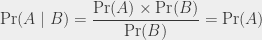
That formula is also pretty useful in the other direction:

because it’s sometimes easier to understand what happens in the context of conditional probabilities than in the context of two non-independent events occurring.

In the next blog post, we’ll talk about random variables 🙂