I worked a bit on Marzipan this week-end, and started playing with bitmap orbits. The idea is the same as for point orbits and line orbits: we look at the iterations of the escaping points, and we look at the distance on the plane between the complex numbers represented by these iterations and a given set on the same plane.
Since my creativity was apparently all used up by trying to make the algorithm work instead of trying to find a nice bitmap to play with, I simply have the name of my project somewhere on an image, as black&white. I pre-compute a distance map to that bitmap (in a very approximate and most probably buggy way right now – something’s not quite right there, but good enough for a first approximation) and I use that distance map to display the points I’m interested in when rendering the fractal.
The very annoying thing is that I do have a bug on the zooming algorithm – things tend to flip and/or to go to weird places. I haven’t been able to track it down yet: it must be said that I’m typically hopeless at handling 2D grids and scaling factors without breaking a neuron or two, and that on top of that, as mentioned previously, I’m probably making my own life miserable by using a non-standard window manager. I’ll probably need to go to KDE or something to debug this thing properly (sigh :/)
Still, in the meantime, I’m not unhappy with the results 🙂
I got half nerd-sniped (by my dad, as it quite often happens) after my blog post on my fractal renderer – “but… your continuous coloring, there… how does it work?”. I had implemented it 8 months ago without really asking myself the question, so after answering “eh, some magic”, I finally got curious for real, and I started digging a bit more into it.
Starting from the Wikipedia article footnotes, I ended up on a couple of articles: Renormalizing the Mandelbrot Escape and Smooth Escape Iteration Counts, as well as smooth iteration count for generalized Mandelbrot sets, that mostly allowed me to piece together some understanding of it. I will admit that my own understanding is still a bit messy/sloppy – my aim here is to try to give some understanding somewhere between “apply this function and you get smooth coloring” and “spectral analysis of eigenvalues in Hilbert spaces” (it’s APPARENTLY related; I’m pretty sure I’ve known at SOME point what this group of words meant, but right now it’s barely a fuzzy concept. Math: if you don’t use it you lose it 🙁 ).
Mandelbrot set and discrete coloring
Before talking about continuous coloring, let me set a few concepts and notations so that we’re on the same page.
We iterate, from a point (where are coordinates on the plane), the sequence , where is a starting constant, typically 0, and we look at the points for which this sequence diverges to infinity or does not. The points for which the sequence does not diverge to infinity (i.e., the sequence is bounded) are part of the Mandelbrot set.
Counting to infinity is, however, a bit long. The first thing we can do is – if we know early that the sequence goes to infinity, we can stop counting: the sequence diverges. We happen to know that, for , the sequence diverges as soon as its magnitude (or equivalently, ). (Note that the minimum value for this to work is .) So we can iterate on every point and, as soon as its magnitude reaches 2, conclude that the point is not in the Mandelbrot set. This process gives another information: the iteration at which this condition is met – which is an indication about how fast the sequence diverges.
That only solves a part of the problem – because by definition, the points for which the sequence is bounded will never stop the process in that model. So the second thing we do is to consider that if a sequence has not diverged after a given, fixed number of iterations, then probably it won’t.
Finally, for every possible number of iterations, we define a color (in a way that eventually makes the result pretty/interesting); we also define a color for points whose sequence does not diverge (and that are considered in the set); and we color each point according to that.
Now the thing with this approach is that the number of iterations tend to gather in “bands” – as in the following picture.
Discrete coloring bands
Smooth coloring
The bands come from the fact that two neighboring pixels “tend to” have the same number of iterations, and hence the same color. If the range of possible values is smooth, and if two neighboring points end up not being associated to the exact same value, and if the palette maps them to different colors, then the coloring should be smooth – even with a fairly reduced palette.
The idea is that we want to represent whether a sequence “barely” reached the escape radius or whether it could have done so almost on the previous iteration, so far it is from the threshold. Ideally, we represent that by a function that goes from 0 to 1, we get a nice smooth range, and that yields a nice smooth coloring.
Now many sources go from this statement to “and now, like a rabbit out of the hat, take and we’re done”. Some of them mumble something about “deriving it from Douady-Hubbard potential“, but it’s not really satisfying either. I gave a quick look to that, and I may revisit the topic eventually, but right now the maths go wayyyy over my head 🙁
Still, the main question I had was “well, if we’re only interested in mapping ‘the space between the bands’, why not just drop a linear operator on that and be done?”. My reasoning was as follows: we know that at iteration , we’re above the radius of convergence , and we were not in the previous iteration, that means that we can bound it. If and are the values of at escape iteration , we have, by definition of , and . To bound from the above, we write (by definition of ), which is less than (by triangular inequality), which is in turn less than .
Hence, our “escape margin” is between 0 and , and we want to map that to something between 0 and 1, so let’s just divide those two things, define my fractional iteration count as and we’re done, right?
Hmmm. It DOES look smooth-er. It’s not… smooth. I have two guesses here. First: the triangular inequality is a bit too rough for my estimate. Second: it may be that I’m generally speaking missing something somewhere. Maybe a bit of both.
Now that’s where the “magic” happens. I’ve read enough on the topic to have some inkling that there’s actual, proper math behind that makes it work, but I’m not able to understand, let alone explain it in simple terms 😉
The fractional iteration count that makes things work is . The best intuition/simplified explanation I’ve seen for this comes from Renormalizing the Mandelbrot Escape, where they have the following quote:
The following simplified and very insightful explanation is provided by Earl L. Hinrichs: “Ignoring the +C in the usual formula, the orbit point grows by Z := Z^2. So we have the progression Z, Z^2, Z^4, Z^8, Z^16, etc. Iteration counting amounts to assigning an integer to these values. Ignoring a multiplier, the log of this sequence is: 1, 2, 4, 8, 16. The log-log is 0, 1, 2, 3, 4 which matches the integer value from the iteration counting. So the appropriate generalization of the discrete iteration counting to a continuous function would be the double log.”
Smooth coloring
So, there. I’m going to leave the topic there for now – that was quite fun to dig into, but I do need more advanced math if I want to dig deeper. It might happen – who knows – but not now 🙂
Around a year ago, I started playing with a small fractal generator that I called Marzipan (because, well, Mandelbrot – basically marzipan, right). Okay, in all fairness, I re-used that name from a previous small fractal generator that I had coded in Javascript several years ago 🙂
It’s primarily (for now) a renderer of colored Mandelbrot sets. The Mandelbrot set is fairly well-known:
Mandelbrot set
This image is a made on a 2D plane whose upper-left coordinate is at (-2, -1) and lower-end coordinate is at (1, 1). For each point (x, y) of this plane, we consider the complex number z = x + yi, we do some operations (called iterations) repeatedly on z, and we see what is the result. If z grows larger and larger (if the sequence of operations diverges), the point z is not in the Mandelbrot set, and we color it grey. If it does not, or if we give up before seeing that it diverges, the point z in in the Mandelbrot set, and we color it black. The longer we wait before deciding that a point is in the set, the more precise the boundary is (because we have “more chances” that it diverges if it is going to diverge).
And it’s technically possible to zoom as much as you want on the border of the set and to get “interesting” results at infinite amount of zoom – every little part of the border has an infinite amount of detail.
Now one of the reason why Mandelbrot (and other similar computation) renderings are quite popular is that they’re colorful and pretty. In particular, I have a fair amount of screen wallpaper coming from Blatte’s Backgrounds, that contain some of this kind of images. The connection between my set above and the colorful images I linked is not a priori obvious.
Enter: coloring algorithms. The idea is to try to represent graphically how the points outside of the set diverge. The first algorithm I implemented was a escape time algorithm: if the point diverges after 5 iterations, color it in a given color, after 6, in an other color, after 50, in yet another color, and so on. And the fastest way to generate a color palette is to just generate it randomly (and to affect one color to each possible number of iterations), which can yield… fairly ugly images 😉
Random coloring of the escape time
A variation of that approach is to affect to each number of iteration a color that is “proportional” (for instance, more or less saturated) to the number of points that actually reach that number of iterations.
Histogram coloring of the escape time
Then the next idea is to go from “discrete coloring” to “continuous coloring” – right now, we have bands of colors that may have some aesthetic quality, but that may not work for what one has in mind in the end. To achieve that, we add a “continuous” component to our iteration computation (so that it’s not integer anymore) and we map it to the color palette.
Continuous coloring of the escape time
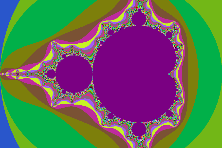
The other coloring algorithm that I started exploring today is coloring by orbit traps. Instead of considering when the iteration escape, we look at how it escapes, and we try to represent that. The first idea is to take an arbitrary, “interesting” point (from an aesthetic point of view, and mostly found by trial and error at this stage), and to look at how close the iterations of the escaping points come to this fixed point). The colored values are the distances to this point. (And the image at the beginning of this post is a (low) zoom from this one 🙂 ) Note: on this one I also tweaked the palette computation to get more contrast. That was fun 🙂
Coloring of the distance to an orbit point (-0.25 + 0.5i)
Generally speaking, this project is also for me a nice visual sandbox to play around – on top of practicing my C++, my goal is to generate pretty images, but that typically requires a fair amount of “quality of life” updates:
a very basic set of command-line options so that I could generate images without hard-coding all the values
quicker than I would have thought: a minimal Qt UI that allows me to zoom and increase/decrease the number of iterations – and right now I kind of feel the need to expand that UI so that it’s… actually useable (being able to change parameters on the UI, re-scaling the window to fit the ratio of the rendered input, that sort of things)
yesterday, I sped up the rendering by… well, adding threads 😛 (via the QtConcurrent library).
Generally speaking, it’s a fun project – and it’s actually something I can go back to quite quickly (once I go over the shock of “urgh C++” – I actually DO like C++, but I did AoC in Go, and it’s a fairly different language) and implement a thing or two here or there, which is nice. For instance, a few months ago, I went “given my current code, can I add support for Julia sets within 10 minutes before going to bed?” and the answer was yes:


 (where
  are coordinates on the plane), the sequence
  , where
  is a starting constant, typically 0, and we look at the points for which this sequence diverges to infinity or does not. The points for which the sequence does not diverge to infinity (i.e., the sequence is bounded) are part of the Mandelbrot set.
  (or equivalently,
  ). (Note that the minimum value for this to work is
  .) So we can iterate on every point and, as soon as its magnitude reaches 2, conclude that the point is not in the Mandelbrot set. This process gives another information: the iteration at which this condition is met – which is an indication about how fast the sequence diverges.
 and we’re done”. Some of them mumble something about “deriving it from
  , we’re above the radius of convergence
  , and we were not in the previous iteration, that means that we can bound it. If
  and
and  are the values of
  and
and  . To bound
  (by definition of
  (by triangular inequality), which is in turn less than
  .
. is between 0 and
  , and we want to map that to something between 0 and 1, so let’s just divide those two things, define my fractional iteration count as
  and we’re done, right?
 . The best intuition/simplified explanation I’ve seen for this comes from