I got half nerd-sniped (by my dad, as it quite often happens) after my blog post on my fractal renderer – “but… your continuous coloring, there… how does it work?”. I had implemented it 8 months ago without really asking myself the question, so after answering “eh, some magic”, I finally got curious for real, and I started digging a bit more into it.

Starting from the Wikipedia article footnotes, I ended up on a couple of articles: Renormalizing the Mandelbrot Escape and Smooth Escape Iteration Counts, as well as smooth iteration count for generalized Mandelbrot sets, that mostly allowed me to piece together some understanding of it. I will admit that my own understanding is still a bit messy/sloppy – my aim here is to try to give some understanding somewhere between “apply this function and you get smooth coloring” and “spectral analysis of eigenvalues in Hilbert spaces” (it’s APPARENTLY related; I’m pretty sure I’ve known at SOME point what this group of words meant, but right now it’s barely a fuzzy concept. Math: if you don’t use it you lose it 😦 ).

Mandelbrot set and discrete coloring

Before talking about continuous coloring, let me set a few concepts and notations so that we’re on the same page.

We iterate, from a point (where are coordinates on the plane), the sequence , where is a starting constant, typically 0, and we look at the points for which this sequence diverges to infinity or does not. The points for which the sequence does not diverge to infinity (i.e., the sequence is bounded) are part of the Mandelbrot set.

Counting to infinity is, however, a bit long. The first thing we can do is – if we know early that the sequence goes to infinity, we can stop counting: the sequence diverges. We happen to know that, for , the sequence diverges as soon as its magnitude (or equivalently, ). (Note that the minimum value for this to work is .) So we can iterate on every point and, as soon as its magnitude reaches 2, conclude that the point is not in the Mandelbrot set. This process gives another information: the iteration at which this condition is met – which is an indication about how fast the sequence diverges.

That only solves a part of the problem – because by definition, the points for which the sequence is bounded will never stop the process in that model. So the second thing we do is to consider that if a sequence has not diverged after a given, fixed number of iterations, then probably it won’t.

Finally, for every possible number of iterations, we define a color (in a way that eventually makes the result pretty/interesting); we also define a color for points whose sequence does not diverge (and that are considered in the set); and we color each point according to that.

Now the thing with this approach is that the number of iterations tend to gather in “bands” – as in the following picture.

Smooth coloring

The bands come from the fact that two neighboring pixels “tend to” have the same number of iterations, and hence the same color. If the range of possible values is smooth, and if two neighboring points end up not being associated to the exact same value, and if the palette maps them to different colors, then the coloring should be smooth – even with a fairly reduced palette.

The idea is that we want to represent whether a sequence “barely” reached the escape radius or whether it could have done so almost on the previous iteration, so far it is from the threshold. Ideally, we represent that by a function that goes from 0 to 1, we get a nice smooth range, and that yields a nice smooth coloring.

Now many sources go from this statement to “and now, like a rabbit out of the hat, take and we’re done”. Some of them mumble something about “deriving it from Douady-Hubbard potential“, but it’s not really satisfying either. I gave a quick look to that, and I may revisit the topic eventually, but right now the maths go wayyyy over my head 😦

Still, the main question I had was “well, if we’re only interested in mapping ‘the space between the bands’, why not just drop a linear operator on that and be done?”. My reasoning was as follows: we know that at iteration , we’re above the radius of convergence , and we were not in the previous iteration, that means that we can bound it. If and are the values of at escape iteration , we have, by definition of , and . To bound from the above, we write (by definition of ), which is less than (by triangular inequality), which is in turn less than .

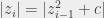
Hence, our “escape margin” is between 0 and , and we want to map that to something between 0 and 1, so let’s just divide those two things, define my fractional iteration count as and we’re done, right?

Hmmm. It DOES look smooth-er. It’s not… smooth. I have two guesses here. First: the triangular inequality is a bit too rough for my estimate. Second: it may be that I’m generally speaking missing something somewhere. Maybe a bit of both.

Now that’s where the “magic” happens. I’ve read enough on the topic to have some inkling that there’s actual, proper math behind that makes it work, but I’m not able to understand, let alone explain it in simple terms 😉

The fractional iteration count that makes things work is . The best intuition/simplified explanation I’ve seen for this comes from Renormalizing the Mandelbrot Escape, where they have the following quote:

The following simplified and very insightful explanation is provided by Earl L. Hinrichs:
“Ignoring the +C in the usual formula, the orbit point grows by Z := Z^2. So we have the progression Z, Z^2, Z^4, Z^8, Z^16, etc. Iteration counting amounts to assigning an integer to these values. Ignoring a multiplier, the log of this sequence is: 1, 2, 4, 8, 16. The log-log is 0, 1, 2, 3, 4 which matches the integer value from the iteration counting. So the appropriate generalization of the discrete iteration counting to a continuous function would be the double log.”

So, there. I’m going to leave the topic there for now – that was quite fun to dig into, but I do need more advanced math if I want to dig deeper. It might happen – who knows – but not now 🙂