All right, I think I explained enough algorithmic complexity (part 1 and part 2) to start with a nice piece, which is to explain what is behind the “Is P equal to NP?” question – also called “P vs NP” problem.
The “P vs NP” problem is one of the most famous open problems, if not the most famous. It’s also part of the Millenium Prize problems, a series of 7 problems stated in 2000: anyone solving one of these problems gets awarded one million dollars. Only one of these problems has been solved, the Poincaré conjecture, proven by Grigori Perelman. He was awarded the Fields medal (roughly equivalent to a Nobel Prize in mathematics) for it, as well as the aforementioned million dollars; he declined both.
But enough history, let’s get into it. P and NP are called “complexity classes”. A complexity class is a set of problems that have common properties. We consider problems (for instance “can I go from point A to point B in my graph with 15 steps or less?”) and to put them in little boxes depending on their properties, in particularity their worst case time complexity (how much time do I need to solve them) and their worst case space complexity (how much memory do I need to solve them).
I explained in the algorithmic complexity blog posts what it meant for an algorithm to run in a given time. Saying that a problem can be/is solved in a given time means that we know how to solve it in that time, which means we have an algorithm that runs in that time and returns the correct solution. To go back to my previous examples, we saw that it was possible to sort a set of elements (books, or other elements) in time . It so happens that, in classical computation models, we can’t do better than . We say that the complexity of sorting is , and we also say that we can sort elements in polynomial time.
A polynomial time algorithm is an algorithm that finishes with a number of steps that is less than , where is the size of the input and an arbitrary number (including very large numbers, as long as they do not depend on ). The name comes from the fact that functions such as , , and are called polynomial functions. Since I can sort elements in time , which is smaller than , sorting is solved in polynomial time. It would also work if I could only sort elements in time , that would also be polynomial. The nice thing with polynomials is that they combine very well. If I make two polynomial operations, I’m still in polynomial time. If I make a polynomial number of polynomial operations, I’m still in polynomial time. The polynomial gets “bigger” (for instance, it goes from to ), but it stays a polynomial.
Now, I need to explain the difference between a problem and an instance of a problem – because I kind of need that level of precision 🙂 A problem regroups all the instances of a problem. If I say “I want to sort my bookshelf”, it’s an instance of the problem “I want to sort an arbitrary bookshelf”. If I’m looking at the length shortest path between two points on a given graph (for example a subway map), it’s an instance of the problem “length of shortest path in a graph”, where we consider all arbitrary graphs of arbitrary size. The problem is the “general concept”, the instance is a “concrete example of the general problem”.
The complexity class P contains all the “decision” problems that can be solved in polynomial time. A decision problem is a problem that can be answered by yes or no. It can seem like a huge restriction: in practice, there are sometimes way to massage the problem so that it can get in that category. Instead of asking for “the length of the shortest path” (asking for the value), I can ask if there is “a path of length less than X” and test that on various X values until I have an answer. If I can do that in a polynomial number of queries (and I can do that for the shortest path question), and if the decision problem can be solved in polynomial time, then the corresponding “value” problem can also be solved in polynomial time. As for an instance of that shortest path decision problem, it can be “considering the map of the Parisian subway, is there a path going from La Motte Piquet Grenelle to Belleville that goes through less than 20 stations?” (the answer is yes) or “in less than 10 stations?” (I think the answer is no).
Let me give another type of a decision problem: graph colorability. I like these kind of examples because I can make some drawings and they are quite easy to explain. Pick a graph, that is to say a bunch of points (vertices) connected by lines (edges). We want to color the vertices with a “proper coloring”: a coloring such that two vertices that are connected by a single edge do not have the same color. The graph colorability problems are problems such as “can I properly color this graph with 2, 3, 5, 12 colors?”. The “value” problem associated to the decision problem is to ask what is the minimum number of colors that I need to color the graph under these constraints.
Let’s go for a few examples – instances of the problem 🙂
A “triangle” graph (three vertices connected with three edges) cannot be colored with only two colors, I need three:
On the other hand, a “square-shaped” graph (four vertices connected as a square by four edges) can be colored with two colors only:
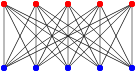
There are graphs with a very large number of vertices and edges that can be colored with only two colors, as long as they follow that type of structure:
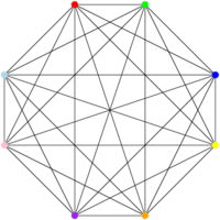
And I can have graphs that require a very large number of colors (one per vertex!) if all the vertices are connected to one another, like this:
And this is where it becomes interesting. We know how to answer in polynomial time (where is of the number of vertices of the graph) to the question “Can this graph be colored with two colors?” for any graph. To decide that, I color an arbitrary vertex of the graph in blue. Then I color all of its neighbors in red – because since the first one is blue, all of its neighbors must be red, otherwise we violate the constraint that no two connected vertices can have the same color. We try to color all the neighbors of the red vertices in blue, and so on. If we manage to color all the vertices with this algorithm, the graph can be colored with two colors – since we just did it! Otherwise, it’s because a vertex has a neighbor that constrains it to be blue (because the neighbor is red) and a neighbor that constrains it to be red (because the neighbor is blue). It is not necessarily obvious to see that it means that the graph cannot be colored with two colors, but it’s actually the case.
I claim that this algorithm is running in polynomial time: why is that the case? The algorithm is, roughly, traversing all the vertices in a certain order and coloring them as it goes; the vertices are only visited once; before coloring a vertex, we check against all of its neighbors, which in the worst case all the other vertices. I hope you can convince yourself that, if we do at most (number of vertices we traverse) times comparisons (maximum number of neighbors for a given vertex), we do at most operations, and the algorithm is polynomial. I don’t want to give much more details here because it’s not the main topic of my post, but if you want more details, ping me in the comments and I’ll try to explain better.
Now, for the question “Can this graph be colored with three colors?”, well… nobody has yet found a polynomial algorithm that allows us to answer the question for any instance of the problem, that is to say for any graph. And, for reasons I’ll explain in a future post, if you find a (correct!) algorithm that allows to answer that question in polynomial time, there’s a fair chance that you get famous, that you get some hate from the cryptography people, and that you win one million dollars. Interesting, isn’t it?
The other interesting thing is that, if I give you a graph that is already colored, and that I tell you “I colored this graph with three colors”, you can check, in polynomial time, that I’m not trying to scam you. You just look at all the edges one after the other and you check that both vertices of the edge are colored with different colors, and you check that there are only three colors on the graph. Easy. And polynomial.
That type of “easily checkable” problems is the NP complexity class. Without giving the formal definition, here’s the idea: a decision problem is in the NP complexity class if, for all instances for which I can answer “yes”, there exists a “proof” that allows me to check that “yes” in polynomial time. This “proof” allows me to answer “I bet you can’t!” by “well, see, I can color that way, it works, that proves that I can do that with three colors” – that is, if the graph is indeed colorable with 3 colors. Note here that I’m not saying anything about how to get that proof – just that if I have it, I can check that it is correct. I also do not say anything about what happens when the instance cannot be colored with three colors. One of the reasons is that it’s often more difficult to prove that something is impossible than to prove that it is possible. I can prove that something is possible by doing it; if I can’t manage to do something, it only proves that I can’t do it (but maybe someone else could).
To summarize:
P is the set of decision problems for which I can answer “yes” or “no” in polynomial time for all instances
NP is the set of decision problems for which, for each “yes” instance, I can get convinced in polynomial time that it is indeed the case if someone provides me with a proof that it is the case.
The next remark is that problems that are in P are also in NP, because if I can answer myself “yes” or “no” in polynomial time, then I can get convinced in polynomial time that the answer is “yes” if it is the case (I just have to run the polynomial time algorithm that answers “yes” or “no”, and to check that it answers “yes”).
The (literally) one-million-dollar question is to know whether all the problems that are in NP are also in P. Informally, does “I can see easily (i.e. in polynomial time) that a problem has a ‘yes’ answer, if I’m provided with the proof” also mean that “I can easily solve that problem”? If that is the case, then all the problems of NP are in P, and since all the problems of P are already in NP, then the P and NP classes contain exactly the same problems, which means that P = NP. If it’s not the case, then there are problems of NP that are not in P, and so P ≠ NP.
The vast majority of maths people think that P ≠ NP, but nobody managed to prove that yet – and many people try.
It would be very, very, very surprising for all these people if someone proved that P = NP. It would probably have pretty big consequences, because that would mean that we have a chance to solve problems that we currently consider as “hard” in “acceptable” times. A fair amount of the current cryptographic operations is based on the fact, not that it is “impossible” to do some operations, but that it’s “hard” to do them, that is to say that we do not know a fast algorithm to do them. In the optimistic case, proving that P = NP would probably not break everything immediately (because it would probably be fairly difficult to apply and that would take time), but we may want to hurry finding a solution. There are a few crypto things that do not rely on the hypothesis that P ≠ NP, so all is not lost either 😉
And the last fun thing is that, to prove that P = NP, it is enough to find a polynomial time algorithm for one of the “NP-hard” problems – of which I’ll talk in a future post, because this one is starting to be quite long. The colorability with three colors is one of these NP-hard problems.
I personally find utterly fascinating that a problem which is so “easy” to get an idea about have such large implications when it comes to its resolution. And I hope that, after you read what I just wrote, you can at least understand, if not share, my fascination 🙂
In the previous episode, I explained two ways to sort books, and I counted the elementary operations I needed to do that, and I estimated the number of operations depending on the number of books that I wanted to sort. In particular, I looked into the best case, worst case and average case for the algorithms, depending on the initial ordering of the input. In this post, I’ll say a bit more about best/worst/average case, and then I’ll refine the notion of algorithmic complexity itself.
The “best case” is typically analyzed the least, because it rarely happens (thank you, Murphy’s Law.) It still gives bounds of what is achievable, and it gives a hint on whether it’s useful to modify the input to get the best case more often.
The “worst case” is the only one that gives guarantees. Saying that my algorithm, in the worst case, executes in a given amount of time, guarantees that it will never take longer – although it can be faster. That type of guarantees is sometimes necessary. In particular, it allows to answer the question of what happens if an “adversary” provides the input, in a way that will make the algorithm’s life as difficult as possible – a question that would interest cryptographers and security people for example. Having guarantees on the worst case means that the algorithm works as desired, even if an adversary tries to make its life as miserable as possible. The drawback of using the worst case analysis is that the “usual” execution time often gets overestimated, and sometimes gets overestimated by a lot.
Looking at the “average case” gives an idea of what happens “normally”. It also gives an idea about what happens if the algorithm is repeated several times on independent data, where both the worst case and the best case can happen. Moreover, there is sometimes ways to avoid the worst cases, so the average case would be more useful in that case. For example, if an adversary gives me the books in an order that makes my algorithm slow, I can compensate that by shuffling the books at the beginning so that the probability of being in a bad case is low (and does not depend on my adversary’s input). The drawback of using the average case analysis is that we lose the guarantee that we have on the worst case analysis.
For my book sorting algorithms, my conclusions were as follows:
For the first sorting algorithm, where I was searching at each step for a place to put the book by scanning all the books that I had inserted so far, I had, in the best case, operations, in the worst case, operations, and in the average case, . operations.
For the second sorting algorithm, where I was grouping book groups two by two, I had, in all cases, operations.
I’m going to draw a figure, because figures are pretty. If the colors are not that clear, the plotted functions and their captions are in the same order.
It turns out that, when talking about complexity, these formulas (, , , ) would not be the ones that I would use in general. If someone asked me about these complexities, I would answer, respectively, that the complexities are , (or “quadratic”), again, and .
This may seem very imprecise, and I’ll admit that the first time I saw this kind of approximations, I was quite irritated. (It was in physics class, so I may not have been in the best of moods either.) Since then, I find it quite handy, and even that it makes sense. The fact that “it makes sense” has a strong mathematical justification. For the people who want some precision, and who are not afraid of things like “limit when x tends to infinity of blah blah”, it’s explained there: http://en.wikipedia.org/wiki/Big_O_notation. It’s vastly above the level of the post I’m currently writing, but I still want to justify a couple of things; be warned that everything that follows is going to be highly non-rigorous.
The first question is what happens to smaller elements of the formulas. The idea is that only keep what “matters” when looking at how the number of operations increases with the number of elements to sort. For example, if I want to sort 750 books, with the “average” case of the first algorithm, I have . For 750 books, the two parts of the sum yield, respectively, 140625 and… 1687. If I want to sort 1000 books, I get 250000 and 2250. The first part of the sum is much larger, and it grows much quicker. If I need to know how much time I need, and I don’t need that much precision, I can pick and discard – already for 1000 books, it contributes less than 1% of the total number of operations.
The second question is more complicated: why do I consider as identical and , or and ? The short answer is that it allows to make running times comparable between several algorithms. To determine which algorithm is the most efficient, it’s nice to be able to compare how they perform. In particular, we look at the “asymptotic” comparison, that is to say what happens when the input of the algorithm contains a very large number of elements (for instance, if I have a lot of books to sort) – that’s where using the fastest algorithm is going to be at most worth it.
To reduce the time that it takes an algorithm to execute, I have two possibilities. Either I reduce the time that each operation takes, or I reduce the number of operations. Suppose that I have a computer that can execute one operation by second, and that I want to sort 100 elements. The first algorithm, which needs operations, finishes after 2500 seconds. The second algorithm, which needs operations, finishes after 1328 seconds. Now suppose that I have a much faster computer to execute the first algorithm. Instead of needing 1 second per operation, it’s 5 times faster, and can execute an operation in 0.2 seconds. That means that I can sort 100 elements in 500 seconds, which is faster than the second algorithm on the slower computer. Yay! Except that, first, if I run the second algorithm of the second computer, I can sort my elements five times faster too, in 265 seconds. Moreover, suppose now that I have 1000 elements to sort. With the first algorithm on the fast computer, I need seconds, and with the second algorithm on the much slower computer, seconds.
That’s the idea behind removing the “multiplying numbers” when estimating complexity. Given an algorithm with a complexity “” and algorithm with a complexity ““, I can put the first algorithm on the fastest computer I can: there will always be a number of elements for which the second algorithm, even on a very slow computer, will be faster than the first one. The number of elements in question can be very large if the difference of speed of the computers is large, but since large numbers are what I am interested in anyway, that’s not a problem.
So when I compare two algorithms, it’s much more interesting to see that one needs “something like ” operations and one needs “something like ” operations than to try to pinpoint the exact constant that multiplies the or the .
Of course, if two algorithms need “something along the lines of operations”, asking for the constant that is multiplying that is a valid question. In practice, it’s not done that often, because unless things are very simple and well-defined (and even then), it’s very hard to determine that constant exactly, depending on how you implement it with a programmation language. It would also require to ask exactly what an operation is. There are “classical” models that allow to define all these things, but linking them to current programming languages and computers is probably not realistic.
Everything that I talked about so far is function of , which is in general the “size of the input”, or the “amount of work that the algorithm has to do”. For books to sort, it would be the number of books. For graph operations, it would be the number of vertices of graphs, and/or the number of edges. Now, as “people who write algorithms”, given an input of size , what do we like, what makes us frown, what makes us run very fast in the other direction?
The “constant time algorithms” and “logarithmic time algorithms” (whose numbers of operations are, respectively, a constant that does not depend on or “something like “) are fairly rare, because with operations (or a constant number of operations), we don’t even have the time to look at the whole input. So when we find an algorithm of that type, we’re very, very happy. A typical example of a logarithmic time algorithm is searching an element in a sorted list. When the list is sorted, it is not necessary to read it completely to find the element that we’re looking for. We can start checking if it’s before or after the middle element, and search in the corresponding part of the list. Then we check if it’s before or after the middle of the new part of the list, and so on.
We’re also very happy when we find a “linear time algorithm” (the number of operations is “something like “). That means that we read the whole input, make a few operations per element of the input, and bam, done. is also usually considered as “acceptable”. It’s an important bound, because it is possible to prove that, in standard algorithmic models (which are quite close to counting “elementary” operations), it is not possible to sort elements faster than with operations in the general case (that is to say, without knowing anything about the elements or the order in which they are). There are a number of algorithms that require, at some point, some sorting: if it is not possible to get rid of the sorting, such an algorithm will also not get below operations.
We start grumbling a bit at , , and to grumble a lot on greater powers of . Algorithms that can run in operations, for some value of (even 1000000), are called “polynomial”. The idea is that, in the same way that a algorithm will eventually be more efficient than a algorithm, with a large enough input, a polynomial algorithm, whatever , will be more efficient than a -operation algorithm. Or than a -operation algorithm. Or even than a -operation algorithm.
In the real life, however, this type of reasoning does have its limits. When writing code, if there is a solution that takes 20 times (or even 2 times) less operations than another, it will generally be the one that we choose to implement. And the asymptotic behavior is only that: asymptotic. It may not apply for the size of the inputs that are processed by our code.
There is an example I like a lot, and I hope you’ll like it too. Consider the problem of multiplying matrices. (For people who never saw matrices: they’re essentially tables of numbers, and you can define how to multiply these tables of numbers. It’s a bit more complicated/complex than multiplying numbers one by one, but not that much more complicated.) (Says the girl who didn’t know how to multiply two matrices before her third year of engineering school, but that’s another story.)
The algorithm that we learn in school allows to multiply to matrices of size with operations. There exists an algorithm that is not too complicated (Strassen algorithm) that works in operations (which is better than ). And then there is a much more complicated algorithm (Coppersmith-Winograd and later) that works in operations. This is, I think, the only algorithm for which I heard SEVERAL theoreticians say “yeah, but really, the constant is ugly” – speaking of the number by which we multiply that to get the “real” number of operations. That constant is not very well-defined (for the reasons mentioned earlier) – we just know that it’s ugly. In practice, as far as I know, the matrix multiplication algorithm that is implemented in “fast” matrix multiplication librairies is Strassen’s or a variation of it, because the constant in the Coppersmith-Winograd algorithm is so huge that the matrices for which it would yield a benefit are too large to be used in practice.
And this funny anecdote concludes this post. I hope it was understandable – don’t hesitate to ask questions or make comments 🙂
There, now that I warmed up by writing a couple of posts where I knew where I wanted to go (a general post about theoretical computer science, and a post to explain what is a logarithm, because it’s always useful). And then I made a small break and talked about intuition, because I needed to gather my thoughts. So now we’re going to enter things that are a little bit more complicated, and that are somewhat more difficult to explain for me too. So I’m going to write, and we’ll see what happens in the end. Add to that that I want to explain things while mostly avoiding the formality of maths that’s by now “natural” to me (but believe me, it required a strong hammer to place it in my head in the first place): I’m not entirely sure about the result of this. I also decided to cut this post in two, because it’s already fairly long. The second one should be shorter.
I already defined an algorithm as a well-defined sequence of operations that can eventually give a result. I’m not going to go much further into the formal definition, because right now it’s not useful. And I’m also going to define algorithmic theory, in a very informal way, as the quantity of resources that I need to execute my algorithm. By resources, I will mostly mean “time”, that is to say the amount of time I need to execute the algorithm; sometimes “space”, that is to say the amount of memory (think of it as the amount of RAM or disk space) that I need to execute my algorithm.
I’m going to take a very common example to illustrate my words: sorting. And, to give a concrete example of my sorting, suppose I have a bookshelf full of books (an utterly absurd proposition). And that it suddenly takes my fancy to want to sort them, say by alphabetical order of their author (and by title for two books by same author). I say that a book A is “before” or “smaller than” a book B if it must be put before in the bookshelf, and that it is “after” or “larger than” the book B if it must be sorted after. With that definition, Asimov’s books are “before” or “smaller than” Clarke’s, which are “before” or “smaller than” Pratchett’s. I’m going to keep this example during the whole post, and I’ll draw parallels to the corresponding algorithmic notions.
Let me first define what I’m talking about. The algorithm I’m studying is the sorting algorithm: that’s the algorithm that allows me to go from a messy bookshelf to a bookshelf whose content is in alphabetical order. The “input” of my algorithm (that is to say, the data that I give to my algorithm for processing), I have a messy bookshelf. The “output” of my algorithm, I have the data that have been processed by my algorithm, that is to say a tidy bookshelf.
I can first observe that, the more books I have, the longer it takes to sort them. There’s two reasons for that. The first is that, if you consider an “elementary” operation of the sort (for instance, put a book in the bookshelf), it’s longer to do that 100 times than 10 times. The second reason is that if you consider what you do for each book, the more books there is, the longer it is. It’s longer to search for the right place to put a book in the midst of 100 books than in the midst of 10.
And that’s precisely what we’re interested in here: how the time that is needed to get a tidy bookshelf grows as a function of the number of books or, generally speaking, how the time necessary to get a sorted sequence of elements depends on the number of elements to sort.
This time depends on the sorting method that is used. For instance, you can choose a very, very long sorting method: while the bookshelf is not sorted, you put everything on the floor, and you put the books back in the bookshelf in a random order. Not sorted? Start again. At the other end of the spectrum, you have Mary Poppins : “Supercalifragilistic”, and bam, your bookshelf is tidy. The Mary Poppins method has a nice particularity: it doesn’t depend on the number of books you have. We say that Mary Poppins executes “in constant time”: whatever the number of books that need to be sorted, they will be within the second. In practice, there’s a reason why Mary Poppins makes people dream: it’s magical, and quite hard to do in reality.
Let’s go back to reality, and to sorting algorithms that are not Mary Poppins. To analyze how the sorting works, I’m considering three elementary operations that I may need while I’m tidying:
comparing two books to see if one should be before or after the other,
add the books to the bookshelf,
and, assuming that my books are set in some order on a table, moving a book from one place to another on the table.
I’m also going to suppose that these three operations take the same time, let’s say 1 second. It wouldn’t be very efficient for a computer, but it would be quite efficient for a human, and it gives some idea. I’m also going to suppose that my bookshelf is somewhat magical (do I have some Mary Poppins streak after all?), that is to say that its individual shelves are self-adapting, and that I have no problem placing a book there without going “urgh, I don’t have space on this shelf anymore, I need to move books on the one below, and that one is full as well, and now it’s a mess”. Similarly: my table is magical, and I have no problem placing a book where I want. Normally, I should ask myself that sort of questions, including from an algorithm point of view (what is the cost of doing that sort of things, can I avoid it by being clever). But since I’m not writing a post about sorting algorithms, but about algorithmic complexity, let’s keep things simple there. (And for those who know what I’m talking about: yeah, I’m aware my model is debatable. It’s a model, it’s my model, I do what I want with it, and my explanations within that framework are valid even if the model itself is debatable.)
First sorting algorithm
Now here’s a first way to sort my books. Suppose I put the contents of my bookshelf on the table, and that I want to add the books one by one. The following scenario is not that realistic for a human who would probably remember where to put a book, but let’s try to imagine the following situation.
I pick a book, I put it in the bookshelf.
I pick another book, I compare it with the first: if it must be put before, I put it before, otherwise after.
I pick a third book. I compare it with the book in the first position on the shelf. If it must be put before, I put it before. If it must be put after, I compare with the book on the second position on the shelf. If it must be before, I put it between both books that are already in the shelf. If it must be put after, I put it as last position.
And so on, until my bookshelf is sorted. For each book that I insert, I compare, in order, with the books that are already there, and I add it between the last book that is “before” it and the first book that is “after” it.
And now I’m asking how much time it takes if I have, say, 100 books, or an arbitrary number of books. I’m going to give the answer for both cases: for 100 books and for books. The time for books will be a function of the number of books, and that’s really what interests me here – or, to be more precise, what will interest me in the second post of this introduction.
The answer is that it depends on the order in which the books were at the start when they were on my table. It can happen (why not) that they were already sorted. Maybe I should have checked before I put everything on the table, it would have been smart, but I didn’t think of it. It so happens that it’s the worst thing that can happen to this algorithm, because every time I want to place a book in the shelf, since it’s after/greater than all the books I put before it, I need to compare it all of the books that I put before. Let’s count:
I put the first book in the shelf. Number of operations: 1.
I compare the second book with the first book. I put it in the shelf. Number of operations: 2.
I compare the third book with the first book. I compare the third book with the second book. I put it in the shelf. Number of operations: 3.
I compare the fourth book with the first book. I compare the fourth book with the second book. I compare the fourth book with the third book. I put it in the shelf. Number of operations: 4.
And so on. Every time I insert a book, I compare it to all the books that were placed before it; when I insert the 50th book, I do 49 comparison operations, plus adding the book in the shelf, 50 operations.
So to insert 100 books, if they’re in order at the beginning, I need 1+2+3+4+5+…+99+100 operations. I’m going to need you to trust me on this if you don’t know it already (it’s easy to prove, but it’s not what I’m talking about right now) that 1+2+3+4+5+…+99+100 is exactly equal to (100 × 101)/2 = 5050 operations (so, a bit less than one hour and a half with 1 operation per second). And if I don’t have 100 books anymore, but books in order, I’ll need operations.
Now suppose that my books were exactly in the opposite order of the order they were supposed to be sorted into. Well, this time, it’s the best thing that can happen with this algorithm, because the first book that I add is always smaller than the ones I put before, so I just need a single comparison.
I put the first book in the shelf. Number of operations: 1.
I compare the second book with the second book. I put it in the shelf. Number of operations: 2.
I compare the third book with the first book. I put it in the shelf. Number of operations: 2.
And so on: I always compare with the first book, it’s always before, and I always have 2 operations.
So if my 100 books are exactly in reverse order, I do 1+2+2+…+2 = 1 + 99 × 2 = 199 operations (so 3 minutes and 19 seconds). And if I have books in reverse order, I need operations.
Alright, we have the “best case” and the “worst case”. Now this is where it gets a bit complicated, because the situation that I’m going to describe is less well-defined, and I’m going to start making approximations everywhere. I’m trying to justify the approximations I’m making, and why they are valid; if I’m missing some steps, don’t hesitate to ask in the comments, I may be missing something myself.
Suppose now that my un-ordered books are in state such that every time I add a book, it’s added roughly in the middle of what has been sorted (I’m saying “roughly” because if I sorted 5 books, I’m going to place the 6th after the book in position 2 or position 3 – positions are integer, I’m not going to place it after the book in position 2.5.) Suppose I insert book number : I’m going to estimate the number of comparisons that I make to , which is greater or equal to the number of comparisons that I actually make. To see that, I distinguish on whether is even or odd. You can show that it works for all numbers; I’m just going to give two examples to explain that indeed there’s a fair chance it works.
If I insert the 6th book, I have already 5 books inserted. If I want to insert it after the book in position 3 (“almost in the middle”), I’m making 4 comparisons (because it’s after the books in positions 1, 2 and 3, but before the book in position 4): we have .
If I insert the 7th book, I already have 6 books inserted, I want to insert it after the 3rd book as well (exactly in the middle); so I also make 4 comparisons (for the same reason), and I have .
Now I’m going to estimate the number of operations I need to sort 100 books, overestimating a little bit, and allowing myself “half-operations”. The goal is not to count exactly, but to get an order of magnitude, which will happen to be greater than the exact number of operations.
Book 1: , plus putting on the shelf, 2.5 operations (I actually don’t need to compare here; I’m just simplifying my end computation.)
Book 2: , plus putting on the shelf, 3 operations (again, here, I have an extra comparison, because I have only one book in the shelf already, but I’m not trying to get an exact count).
Book 3: , plus putting on the shelf, 3.5 operations.
Book 4: , plus putting on the shelf, 4 operations.
If I continue like that and I re-order my computations a bit, I have, for 100 books:
which yields roughly 45 minutes.
The first element of my sum is from the that I have in all my comparison computations. The first 100 comes from the “1” that I add every time I count the comparisons (and I do that 100 times); the second “100” comes from the “1” that I do every time I count putting the book in the shelf, which I also do 100 times.
That 2725 is a bit overestimated, but “not that much”: for the first two books, I’m counting exactly 2.5 comparisons too much; for the others, I have at most 0.5 comparisons too much. Over 100 books, I have at most extra operations; the exact number of operations is between 2673 and 2725 (between 44 and 45 minutes). I could do thing a little more precisely, but we’ll see in what follows (in the next post) why it’s not very interesting.
If I’m counting for books, my estimation is
It is possible to prove (but that would really be over the top here) that this behaviour is roughly he one that you get when you have books in a random order. The idea is that if my books are in a random order, I will insert some around the beginning, some around the end, and so “on average” roughly in the middle.
Another sorting algorithm
Now I’m going to explain another sorting method, which is probably less easy to understand, but which is probably the easiest way for me to continue my argument.
Let us suppose, this time, that I want to sort 128 books instead of 100, because it’s a power of 2, and it makes my life easier for my concrete example. And I didn’t think about it before, and I’m too lazy to go back to the previous example to run it for 128 books instead of 100.
Suppose that all my books directly on the table, and I’m going to make “groups” before putting my books in the bookshelf. And I’m going to make these groups in a somewhat weird, but efficient fashion.
First, I combine my books two by two. I take two books, I compare them, I put the smaller one (the one that is before in alphabetical order) on the left, and the larger one on the right. At the end of this operation, I have 64 groups of two books, and for each group, a small book on the left, and a large book on the right. To do this operation, I had to make 64 comparisons, and 128 moves of books (I suppose that I always move books, if only to have them in hand and read the authors/titles).
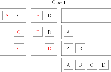
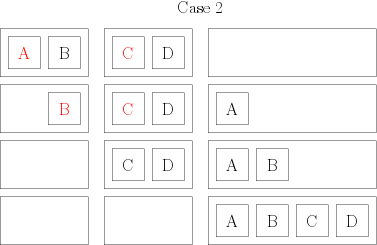
Then, I take my groups of two books, and I combine them again so that I have groups of 4 books, still in order. To do that, I compare the first two books of the group; the smaller of both becomes the first book of my group of 4. Then, I compare the remaining book of the group of 2 from which I picked the first book, and I put the smaller one in position 2 of my group of 4. There, I have two possibilities. Either I have one book in each of my initial groups of 2: in that case, I compare them, and I put them in order in my group of 4. or I still have a full group of two: so I just have to add them at the end of my new group, and I have an ordered group of 4. Here are two little drawings to distinguish both cases: each square represents a book whose author starts by the indicated letter; each rectangle represents my groups of books (the initial groups of two and the final group of 4), and the red elements are the ones that are compared at each step.
So, for each group of 4 that I create, I need to make 4 moves and 2 or 3 comparisons. I end up with 32 groups of 4 books; in the end, to make combine everything into 32 groups of 4 books, I make 32 × 4 = 128 moves and between 32 × 2 = 64 and 32 × 3 = 96 comparisons.
Then, I create 16 groups of 8 books, still by comparing the first element of each group of books and by creating a common, sorted group. To combine two groups of 4 books, I need 8 moves and between 4 and 7 comparisons. I’m not going to get into how exactly to get these numbers: the easiest way to see that is to enumerate all the cases, and while it’s still feasible for groups of 4 books, it’s quite tedious. So to create 16 groups of 8 books, I need to do 16×8 moves and between 16×4 = 64 and 16×7 = 112 comparisons.
I continue like that until I have 2 groups of 64 books, which I combine (directly in the bookshelf to gain some time) to get a sorted group of books.
Now, how much time does that take me? First, let me give an estimation for 128 books, and then we’ll see what happens for books. First, we evaluate the number of comparisons when combining two groups of books. I claim that to combine two groups of elements into a larger group of elements, I need at most comparisons. To see that: every time I place a book in the larger group, it’s either because I compared it to another one (and made a single comparison at that step), or because one of my groups is empty (and there I would make no comparison at all). Since I have a total of books, I make at most comparisons. I also move books to combine my groups. Moreover, for each “overall” step (taking all the groups and combining them two by two), I do overall 128 moves – because I have 128 books, and each of them is in exactly one “small” group at the beginning and ends up in one “large” group at the end. So, for each “overall” step of merging, I’m doing at most 128 comparisons and 128 moves.
Now I need to count the number of overall steps. For 128 books, I do the following:
Combine 128 groups of 1 book into 64 groups of 2 books
Combine 64 groups of 2 books into 32 groups of 4 books
Combine 32 groups of 4 books into 16 groups of 8 books
Combine 16 groups of 8 books into 8 groups of 16 books
Combine 8 groups of 16 books into 4 groups of 32 books
Combine 4 groups of 32 books into 2 groups of 64 books
Combine 2 groups of 64 books into 1 group of 128 books
So I have 7 “overall” steps. For each of these steps, I have 128 moves, and at most 128 comparisons, so at most 7×(128 + 128) = 1792 operations – that’s a bit less than half an hour. Note that I didn’t make any hypothesis here on the initial order of the books. Compare that to the 5050 operations for the “worst case” of the previous computation, or with the ~2700 operations of the “average” case (those numbers were also counted for 100 books; for 128 books we’d have 8256 operations for the worst case and ~4300 with the average case).
Now what about the formula for books? I think we can agree that for each overall step of group combining, we move books, and that we do at most comparisons (because each comparison is associated to putting a book in a group). So, for each overall step, I’m doing at most comparisons. Now the question is: how many steps do we need? And that’s where my great post about logarithms (cough) gets useful. Can you see the link with the following figure?
What if I tell you that the leaves are the books in a random order before the first step? Is that any clearer? The leaves represent “groups of 1 book”. Then the second level represents “groups of two books”, the third represent “groups of 4 books”, and so on, until we get a single group that contains all the books. And the number of steps is exactly equal to the logarithm (in base 2) of the number of books, which corresponds to the “depth” (the number of levels) of the tree in question.
So to conclude, for books, I have, in the model I defined, at most operations.
There, I’m going to stop here for this first post. In the next post, I’ll explain why I didn’t bother too much with exactly exact computations, and why one of the sentences I used to pronounce quite often was “bah, it’s a constant, I don’t care” (and also why sometimes we actually do care).
I hope this post was understandable so far; otherwise don’t hesitate to grumble, ask questions, and all that sort of things. As for me, I found it very fun to write all this 🙂 (And, six years later, I also had fun translating it 🙂 )


 operations, in the worst case,
  operations, and in the average case,
  . operations.
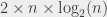 operations.
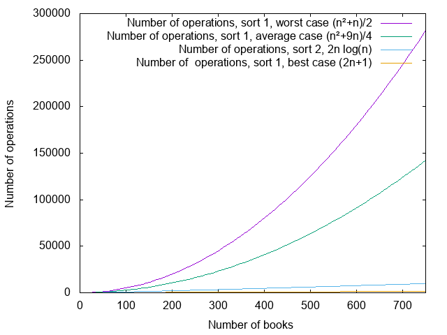
 . For 750 books, the two parts of the sum yield, respectively, 140625 and… 1687. If I want to sort 1000 books, I get 250000 and 2250. The first part of the sum is much larger, and it grows much quicker. If I need to know how much time I need, and I don’t need that much precision, I can pick
  and discard
  – already for 1000 books, it contributes less than 1% of the total number of operations.
 and
and  seconds, and with the second algorithm on the much slower computer,
  seconds.
 “) are fairly rare, because with
  , and to grumble a lot on greater powers of
  -operation algorithm. Or than a
  -operation algorithm. Or even than a
  -operation algorithm.
 with
with  operations (which is better than
  operations. This is, I think, the only algorithm for which I heard SEVERAL theoreticians say “yeah, but really, the constant is ugly” – speaking of the number by which we multiply that
  operations.
 operations.
 : I’m going to estimate the number of comparisons that I make to
  , which is greater or equal to the number of comparisons that I actually make. To see that, I distinguish on whether
  .
. .
. , plus putting on the shelf, 2.5 operations (I actually don’t need to compare here; I’m just simplifying my end computation.)
 , plus putting on the shelf, 3 operations (again, here, I have an extra comparison, because I have only one book in the shelf already, but I’m not trying to get an exact count).
 , plus putting on the shelf, 3.5 operations.
 , plus putting on the shelf, 4 operations.
 that I have in all my comparison computations. The first 100 comes from the “1” that I add every time I count the comparisons (and I do that 100 times); the second “100” comes from the “1” that I do every time I count putting the book in the shelf, which I also do 100 times.
 extra operations; the exact number of operations is between 2673 and 2725 (between 44 and 45 minutes). I could do thing a little more precisely, but we’ll see in what follows (in the next post) why it’s not very interesting.
 elements, I need at most
  comparisons. Now the question is: how many steps do we need? And that’s where my
 operations.