Note: this is the translation of a post that was originally published in French: Introduction à la complexité algorithmique – 1/2.
There, now that I warmed up by writing a couple of posts where I knew where I wanted to go (a general post about theoretical computer science, and a post to explain what is a logarithm, because it’s always useful). And then I made a small break and talked about intuition, because I needed to gather my thoughts. So now we’re going to enter things that are a little bit more complicated, and that are somewhat more difficult to explain for me too. So I’m going to write, and we’ll see what happens in the end. Add to that that I want to explain things while mostly avoiding the formality of maths that’s by now “natural” to me (but believe me, it required a strong hammer to place it in my head in the first place): I’m not entirely sure about the result of this. I also decided to cut this post in two, because it’s already fairly long. The second one should be shorter.
I already defined an algorithm as a well-defined sequence of operations that can eventually give a result. I’m not going to go much further into the formal definition, because right now it’s not useful. And I’m also going to define algorithmic theory, in a very informal way, as the quantity of resources that I need to execute my algorithm. By resources, I will mostly mean “time”, that is to say the amount of time I need to execute the algorithm; sometimes “space”, that is to say the amount of memory (think of it as the amount of RAM or disk space) that I need to execute my algorithm.
I’m going to take a very common example to illustrate my words: sorting. And, to give a concrete example of my sorting, suppose I have a bookshelf full of books (an utterly absurd proposition). And that it suddenly takes my fancy to want to sort them, say by alphabetical order of their author (and by title for two books by same author). I say that a book A is “before” or “smaller than” a book B if it must be put before in the bookshelf, and that it is “after” or “larger than” the book B if it must be sorted after. With that definition, Asimov’s books are “before” or “smaller than” Clarke’s, which are “before” or “smaller than” Pratchett’s. I’m going to keep this example during the whole post, and I’ll draw parallels to the corresponding algorithmic notions.
Let me first define what I’m talking about. The algorithm I’m studying is the sorting algorithm: that’s the algorithm that allows me to go from a messy bookshelf to a bookshelf whose content is in alphabetical order. The “input” of my algorithm (that is to say, the data that I give to my algorithm for processing), I have a messy bookshelf. The “output” of my algorithm, I have the data that have been processed by my algorithm, that is to say a tidy bookshelf.
I can first observe that, the more books I have, the longer it takes to sort them. There’s two reasons for that. The first is that, if you consider an “elementary” operation of the sort (for instance, put a book in the bookshelf), it’s longer to do that 100 times than 10 times. The second reason is that if you consider what you do for each book, the more books there is, the longer it is. It’s longer to search for the right place to put a book in the midst of 100 books than in the midst of 10.
And that’s precisely what we’re interested in here: how the time that is needed to get a tidy bookshelf grows as a function of the number of books or, generally speaking, how the time necessary to get a sorted sequence of elements depends on the number of elements to sort.
This time depends on the sorting method that is used. For instance, you can choose a very, very long sorting method: while the bookshelf is not sorted, you put everything on the floor, and you put the books back in the bookshelf in a random order. Not sorted? Start again. At the other end of the spectrum, you have Mary Poppins : “Supercalifragilistic”, and bam, your bookshelf is tidy. The Mary Poppins method has a nice particularity: it doesn’t depend on the number of books you have. We say that Mary Poppins executes “in constant time”: whatever the number of books that need to be sorted, they will be within the second. In practice, there’s a reason why Mary Poppins makes people dream: it’s magical, and quite hard to do in reality.
Let’s go back to reality, and to sorting algorithms that are not Mary Poppins. To analyze how the sorting works, I’m considering three elementary operations that I may need while I’m tidying:
- comparing two books to see if one should be before or after the other,
- add the books to the bookshelf,
- and, assuming that my books are set in some order on a table, moving a book from one place to another on the table.
I’m also going to suppose that these three operations take the same time, let’s say 1 second. It wouldn’t be very efficient for a computer, but it would be quite efficient for a human, and it gives some idea. I’m also going to suppose that my bookshelf is somewhat magical (do I have some Mary Poppins streak after all?), that is to say that its individual shelves are self-adapting, and that I have no problem placing a book there without going “urgh, I don’t have space on this shelf anymore, I need to move books on the one below, and that one is full as well, and now it’s a mess”. Similarly: my table is magical, and I have no problem placing a book where I want. Normally, I should ask myself that sort of questions, including from an algorithm point of view (what is the cost of doing that sort of things, can I avoid it by being clever). But since I’m not writing a post about sorting algorithms, but about algorithmic complexity, let’s keep things simple there. (And for those who know what I’m talking about: yeah, I’m aware my model is debatable. It’s a model, it’s my model, I do what I want with it, and my explanations within that framework are valid even if the model itself is debatable.)
First sorting algorithm
Now here’s a first way to sort my books. Suppose I put the contents of my bookshelf on the table, and that I want to add the books one by one. The following scenario is not that realistic for a human who would probably remember where to put a book, but let’s try to imagine the following situation.
- I pick a book, I put it in the bookshelf.
- I pick another book, I compare it with the first: if it must be put before, I put it before, otherwise after.
- I pick a third book. I compare it with the book in the first position on the shelf. If it must be put before, I put it before. If it must be put after, I compare with the book on the second position on the shelf. If it must be before, I put it between both books that are already in the shelf. If it must be put after, I put it as last position.
- And so on, until my bookshelf is sorted. For each book that I insert, I compare, in order, with the books that are already there, and I add it between the last book that is “before” it and the first book that is “after” it.
And now I’m asking how much time it takes if I have, say, 100 books, or an arbitrary number of books. I’m going to give the answer for both cases: for 100 books and for 
The answer is that it depends on the order in which the books were at the start when they were on my table. It can happen (why not) that they were already sorted. Maybe I should have checked before I put everything on the table, it would have been smart, but I didn’t think of it. It so happens that it’s the worst thing that can happen to this algorithm, because every time I want to place a book in the shelf, since it’s after/greater than all the books I put before it, I need to compare it all of the books that I put before. Let’s count:
- I put the first book in the shelf. Number of operations: 1.
- I compare the second book with the first book. I put it in the shelf. Number of operations: 2.
- I compare the third book with the first book. I compare the third book with the second book. I put it in the shelf. Number of operations: 3.
- I compare the fourth book with the first book. I compare the fourth book with the second book. I compare the fourth book with the third book. I put it in the shelf. Number of operations: 4.
- And so on. Every time I insert a book, I compare it to all the books that were placed before it; when I insert the 50th book, I do 49 comparison operations, plus adding the book in the shelf, 50 operations.
So to insert 100 books, if they’re in order at the beginning, I need 1+2+3+4+5+…+99+100 operations. I’m going to need you to trust me on this if you don’t know it already (it’s easy to prove, but it’s not what I’m talking about right now) that 1+2+3+4+5+…+99+100 is exactly equal to (100 × 101)/2 = 5050 operations (so, a bit less than one hour and a half with 1 operation per second). And if I don’t have 100 books anymore, but 
Now suppose that my books were exactly in the opposite order of the order they were supposed to be sorted into. Well, this time, it’s the best thing that can happen with this algorithm, because the first book that I add is always smaller than the ones I put before, so I just need a single comparison.
- I put the first book in the shelf. Number of operations: 1.
- I compare the second book with the second book. I put it in the shelf. Number of operations: 2.
- I compare the third book with the first book. I put it in the shelf. Number of operations: 2.
- And so on: I always compare with the first book, it’s always before, and I always have 2 operations.
So if my 100 books are exactly in reverse order, I do 1+2+2+…+2 = 1 + 99 × 2 = 199 operations (so 3 minutes and 19 seconds). And if I have 
Alright, we have the “best case” and the “worst case”. Now this is where it gets a bit complicated, because the situation that I’m going to describe is less well-defined, and I’m going to start making approximations everywhere. I’m trying to justify the approximations I’m making, and why they are valid; if I’m missing some steps, don’t hesitate to ask in the comments, I may be missing something myself.
Suppose now that my un-ordered books are in state such that every time I add a book, it’s added roughly in the middle of what has been sorted (I’m saying “roughly” because if I sorted 5 books, I’m going to place the 6th after the book in position 2 or position 3 – positions are integer, I’m not going to place it after the book in position 2.5.) Suppose I insert book number 

If I insert the 6th book, I have already 5 books inserted. If I want to insert it after the book in position 3 (“almost in the middle”), I’m making 4 comparisons (because it’s after the books in positions 1, 2 and 3, but before the book in position 4): we have 
If I insert the 7th book, I already have 6 books inserted, I want to insert it after the 3rd book as well (exactly in the middle); so I also make 4 comparisons (for the same reason), and I have 
Now I’m going to estimate the number of operations I need to sort 100 books, overestimating a little bit, and allowing myself “half-operations”. The goal is not to count exactly, but to get an order of magnitude, which will happen to be greater than the exact number of operations.
- Book 1:
, plus putting on the shelf, 2.5 operations (I actually don’t need to compare here; I’m just simplifying my end computation.)
- Book 2:
, plus putting on the shelf, 3 operations (again, here, I have an extra comparison, because I have only one book in the shelf already, but I’m not trying to get an exact count).
- Book 3:
, plus putting on the shelf, 3.5 operations.
- Book 4:
, plus putting on the shelf, 4 operations.
If I continue like that and I re-order my computations a bit, I have, for 100 books:

which yields roughly 45 minutes.
The first element of my sum is from the 
That 2725 is a bit overestimated, but “not that much”: for the first two books, I’m counting exactly 2.5 comparisons too much; for the others, I have at most 0.5 comparisons too much. Over 100 books, I have at most 
If I’m counting for

It is possible to prove (but that would really be over the top here) that this behaviour is roughly he one that you get when you have books in a random order. The idea is that if my books are in a random order, I will insert some around the beginning, some around the end, and so “on average” roughly in the middle.
Another sorting algorithm
Now I’m going to explain another sorting method, which is probably less easy to understand, but which is probably the easiest way for me to continue my argument.
Let us suppose, this time, that I want to sort 128 books instead of 100, because it’s a power of 2, and it makes my life easier for my concrete example. And I didn’t think about it before, and I’m too lazy to go back to the previous example to run it for 128 books instead of 100.
Suppose that all my books directly on the table, and I’m going to make “groups” before putting my books in the bookshelf. And I’m going to make these groups in a somewhat weird, but efficient fashion.
First, I combine my books two by two. I take two books, I compare them, I put the smaller one (the one that is before in alphabetical order) on the left, and the larger one on the right. At the end of this operation, I have 64 groups of two books, and for each group, a small book on the left, and a large book on the right. To do this operation, I had to make 64 comparisons, and 128 moves of books (I suppose that I always move books, if only to have them in hand and read the authors/titles).
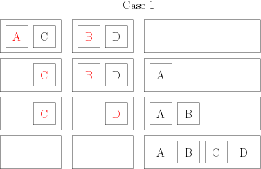
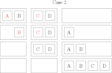
Then, I take my groups of two books, and I combine them again so that I have groups of 4 books, still in order. To do that, I compare the first two books of the group; the smaller of both becomes the first book of my group of 4. Then, I compare the remaining book of the group of 2 from which I picked the first book, and I put the smaller one in position 2 of my group of 4. There, I have two possibilities. Either I have one book in each of my initial groups of 2: in that case, I compare them, and I put them in order in my group of 4. or I still have a full group of two: so I just have to add them at the end of my new group, and I have an ordered group of 4. Here are two little drawings to distinguish both cases: each square represents a book whose author starts by the indicated letter; each rectangle represents my groups of books (the initial groups of two and the final group of 4), and the red elements are the ones that are compared at each step.
So, for each group of 4 that I create, I need to make 4 moves and 2 or 3 comparisons. I end up with 32 groups of 4 books; in the end, to make combine everything into 32 groups of 4 books, I make 32 × 4 = 128 moves and between 32 × 2 = 64 and 32 × 3 = 96 comparisons.
Then, I create 16 groups of 8 books, still by comparing the first element of each group of books and by creating a common, sorted group. To combine two groups of 4 books, I need 8 moves and between 4 and 7 comparisons. I’m not going to get into how exactly to get these numbers: the easiest way to see that is to enumerate all the cases, and while it’s still feasible for groups of 4 books, it’s quite tedious. So to create 16 groups of 8 books, I need to do 16×8 moves and between 16×4 = 64 and 16×7 = 112 comparisons.
I continue like that until I have 2 groups of 64 books, which I combine (directly in the bookshelf to gain some time) to get a sorted group of books.
Now, how much time does that take me? First, let me give an estimation for 128 books, and then we’ll see what happens for 

Now I need to count the number of overall steps. For 128 books, I do the following:
- Combine 128 groups of 1 book into 64 groups of 2 books
- Combine 64 groups of 2 books into 32 groups of 4 books
- Combine 32 groups of 4 books into 16 groups of 8 books
- Combine 16 groups of 8 books into 8 groups of 16 books
- Combine 8 groups of 16 books into 4 groups of 32 books
- Combine 4 groups of 32 books into 2 groups of 64 books
- Combine 2 groups of 64 books into 1 group of 128 books
So I have 7 “overall” steps. For each of these steps, I have 128 moves, and at most 128 comparisons, so at most 7×(128 + 128) = 1792 operations – that’s a bit less than half an hour. Note that I didn’t make any hypothesis here on the initial order of the books. Compare that to the 5050 operations for the “worst case” of the previous computation, or with the ~2700 operations of the “average” case (those numbers were also counted for 100 books; for 128 books we’d have 8256 operations for the worst case and ~4300 with the average case).
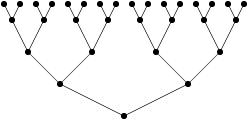
Now what about the formula for 

What if I tell you that the leaves are the books in a random order before the first step? Is that any clearer? The leaves represent “groups of 1 book”. Then the second level represents “groups of two books”, the third represent “groups of 4 books”, and so on, until we get a single group that contains all the books. And the number of steps is exactly equal to the logarithm (in base 2) of the number of books, which corresponds to the “depth” (the number of levels) of the tree in question.
So to conclude, for 
There, I’m going to stop here for this first post. In the next post, I’ll explain why I didn’t bother too much with exactly exact computations, and why one of the sentences I used to pronounce quite often was “bah, it’s a constant, I don’t care” (and also why sometimes we actually do care).
I hope this post was understandable so far; otherwise don’t hesitate to grumble, ask questions, and all that sort of things. As for me, I found it very fun to write all this 🙂 (And, six years later, I also had fun translating it 🙂 )

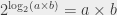
 (read “two to the power of

 . And, well, in the same way, I can define a logarithm that would be the inverse of this


 ,
,  (because
  ); the logarithm base 10 of all the numbers between 10 and 100 is between 1 and 2. In the same way, you can say that the logarithm base 10 of 14578 is between 4 and 5, because 14578 is between
  and
and  , which allows to conclude on the value of the logarithm. (I’m hiding a number of things here, including the reasons that make that reasoning actually correct.)
 to
to  , and on a “normal” scale, you wouldn’t be able to distinguish between
  . You can however use a logarithmic scale, so that you represent with the same amount of space “things that happen between
  (corresponding to the power at which I raise
 (corresponding to… okay, you get the idea) if I want to. It’s less “intuitive” than when looking at the explanation with the tree and the number of levels (because it’s pretty hard to draw
  ,
,  and
and  :
:
 . Here, I feel that it’s possible someone just read that and went “wait, what?”. As far as powers go, there is a “special” one: the powers of
  .
.  has its own name and its own notation: it’s the exponential function, and
  . It’s special because of an interesting property: it is equal to its derivative. And because the exponential function is often used, its inverse, the “natural logarithm” (logarithm in base
  . It’s also been
  and use
  .
.  . Formally, we write that

 . And you can represent the natural logarithm of any value (greater than 1) by the area of the zone between the x-axis and the
  for all
  ).
).

 , then
  , putting everything together yields the first result. The second equality (with the minuses) can be derived in exactly the same way (and left as an exercise to the reader 😉 ).
 (where
  are coordinates on the plane), the sequence
  , where
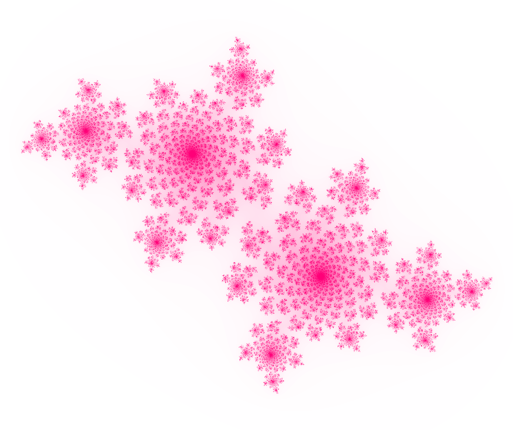
  is a starting constant, typically 0, and we look at the points for which this sequence diverges to infinity or does not. The points for which the sequence does not diverge to infinity (i.e., the sequence is bounded) are part of the Mandelbrot set.
  (or equivalently,
  ). (Note that the minimum value for this to work is
  .) So we can iterate on every point and, as soon as its magnitude reaches 2, conclude that the point is not in the Mandelbrot set. This process gives another information: the iteration at which this condition is met – which is an indication about how fast the sequence diverges.
 and we’re done”. Some of them mumble something about “deriving it from
  , and we were not in the previous iteration, that means that we can bound it. If
  and
and  are the values of
  and
and  . To bound
 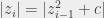 (by definition of
  (by triangular inequality), which is in turn less than
  .
. is between 0 and
  , and we want to map that to something between 0 and 1, so let’s just divide those two things, define my fractional iteration count as
  and we’re done, right?
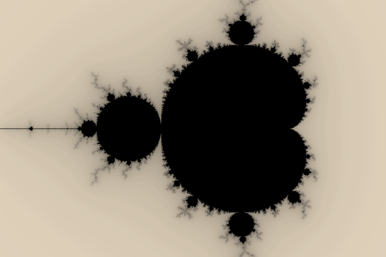
 . The best intuition/simplified explanation I’ve seen for this comes from