Balise's Blog

Intro to probability theory – part 1

Published on 10 February 201910 February 2019 by Balise2 Comments

Ce billet est la traduction d’un billet écrit en français ici : Probabilités – partie 1

I’m eventually going to talk a bit about random algorithms, but before I do that, I need to talk about probability theory so that everyone is speaking the same language.

Probability theory is a bit annoying, because probability is something that many people use fairly often in their daily life, but it can be awfully counter-intuitive. That, or human beings suck at probability theory – also a possibility.

I kind of don’t want to formally define probability (“given a universe $\Omega$ , events”, blah blah blah… yeah, no, don’t want to do that), I’m going to try to explain things in a handwavy way, and hope for the best.

First, let me assume that everything I’m talking about here – unless mentioned otherwise explicitly – has “usual” properties: dice are not loaded, coins are real coins, etc.

Let us start with a classical example. If I flip a coin, what is the probability that it shows heads when it lands? The answer is 1/2: I have two possible events (the coin can show heads or tails), and they both have the same probability of occurring. Same thing if I roll a 6-sided die: the probability that it shows 4 is 1/6; I have six possible events that all have the same probability of occurring. In general, I’ll say that if I do an experiment (flipping a coin, rolling a die) that has $k$ possible outcomes, and that all of these outcomes have the same probability (“chance of happening”), then the probability of each of these outcomes (“events”) is $\displaystyle \frac 1 k$ .

It can happen that all the possible outcomes don’t have the same probability, but there are a few non-negotiable rules. A probability is always a number between 0 and 1. An event that never occurs has probability 0; an event that always occurs has probability 1. If I find a coin with two “heads” sides, and I flip it, it shows “heads” with probability 1 and “tails” with probability 0. Moreover, the sum of all the probabilities of all the possible outcomes of a given experience sums to 1. If I have $k$ events that have the same probability, we indeed have $\displaystyle k \times \frac 1 k = 1$ . If I have a die with three sides 1, two sides 2 and one side 3, the probability that it shows 1 is $\displaystyle \frac 3 6$ , the probability that it shows 2 is $\displaystyle \frac 2 6$ , and the probability that it shows 3 is $\displaystyle \frac 1 6$ ; the sum of all these is $\displaystyle \frac 3 6 + \frac 2 6 + \frac 1 6 = 1$ .

Now it gets a bit trickier. What is the probability that a (regular) 6-sided die shows 3 or 5? Well, the probability that it shows 3 is $\displaystyle \frac 1 6$ ; the probability that it shows 5 is $\displaystyle \frac 1 6$ , and the probability that it shows 3 or 5 is $\displaystyle \frac 1 6 + \frac 1 6 = \frac 1 3$ . But summing the individual probabilities only works if the events are exclusive, that is to say they cannot both be true at the same time: if I rolled a 5, then I can’t have a 3, and vice-versa.

It does not work if two events can both occur at the same time (non-exclusively). For instance, consider that flip a coin and roll a die, and I look at the probability that the coin lands on tails or that the die lands on 6. Then I CANNOT say that it’s equal to the probability of the coin landing on tails – $\displaystyle \frac 1 2$ -, plus the probability that the die lands on 6 – $\displaystyle \frac 1 6$ – for a total of $\displaystyle \frac 2 3$ . A way to see that is to tweak the experiment a bit to see that it doesn’t work all the time. For example, the probability that the die lands on 1,2, 3 or 4 is $\displaystyle \frac 4 6 = \frac 2 3$ . The probability that the coin lands on tails is $\displaystyle \frac 1 2$ . And it’s not possible that the combined probability of these two events (the die lands on 1, 2, 3 or 4, or the coin lands on tails) is the sum of both probabilities, because that would yield $\displaystyle \frac 2 3 + \frac 1 2 = \frac 7 6$ , which is greater than 1. (And a probability is always less or equal to 1).

What is true, though, is that if I have events $A$ and $B$ , then

$\Pr(A \cup B) \leq \Pr(A) + \Pr(B)$

where $\Pr(A)$ is “probability that $A$ occurs”, $\Pr(B)$ is “probability that $B$ occurs” and $\Pr(A \cup B)$ is “probability that $A$ occurs or that $B$ occurs”. Or, in a full sentence: the probability of the union of two events (event $A$ occurs or event $B$ occurs) is always less than or equal to the sum of the probabilities of both events. You can extend this to more events: the probability of the union of several events is less than or equal to the sum of the probabilities of the individual events. It may not seem very deep a result, but in practice it’s used quite often under the name “union bound”. The union bound does not necessarily yield interesting results. For the case “the die lands on 1, 2, 3 or 4, or the coin lands on tails”, it yields a bound at $\displaystyle \frac 7 6$ … and we already had a better bound by the fact that the probability is always less than 1. It is slightly more useful to bound the probability that the die lands on a 6 or that the coin lands on tails: we know that the probability is less than $\displaystyle \frac 2 3$ . When analyzing random algorithms, the union bound is often pretty useful, because the probabilities that we consider are often pretty small, and we can add a lot of them before the bound stops making sense. The union bound is often not enough to make a useful conclusion, but it’s very often a useful tool as a step of a proof.

For the example that I’ve been using so far, the best tool (because it gives an exact result) is the inclusion-exclusion principle. For two events $A$ and $B$ , it’s stated as follows:

$\Pr(A \cup B) = \Pr(A) + \Pr(B) - \Pr(A \cap B)$

with the same notation as previously, and $\Pr(A \cap B)$ representing the probability that both events $A$ and $B$ occur. In a sentence: the probability that $A$ or $B$ occur is equals to the sum of the probabilities that either of them occurs, minus the probability that both $A$ and $B$ occur at the same time. The idea is that, if two events can occur at the same time, that probability is counted twice when summing the probabilities. It may be clearer with a small drawing (also known as Venn diagram):

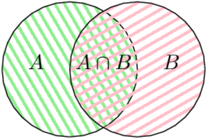
If I count everything that is in the green area (corresponding to event $A$ ), and everything that is in the pink area (corresponding to event $B$ ), I count twice what is both in the green and pink area; if I want to have the correct result, I need to remove once what is common to both areas.

Now the question becomes – how to compute the probability of two events arriving at the same time? There’s the easy case, and the not so easy case. In the easy case, the events are independent: the probability that one occurs has no impact on the probability that the other one occurs. It’s is true (although not necessarily intuitive) if one is working with dice and coins and considering their individual results, but it’s a notion that requires a lot of care to apply (it’s not true anymore if I’m interested in the individual results and the sum of two dice, for example). Proving that two events are independent can be pretty complicated, and handling computations when they are not… as well.

When two events are independent, we have:

$\Pr(A \cap B) = \Pr(A) \times \Pr(B)$

that is to say that the probability that both events occur is equal to the product of the probabilities of both events. If I’m flipping a coin and rolling a die, the coin landing on tails has no impact on the die landing on 6. Both events are independent; the probability that both events occur is consequently $\displaystyle \frac 1 2 \times \frac 1 6 = \frac{1}{12}$ . Observe that this probability is smaller than $\displaystyle \frac 1 2$ and smaller than $\displaystyle \frac 1 6$ . It’s “obvious” since a probability is smaller than one, and that consequently multiplying two probabilities together yields a result that is smaller than both. Another way to see that is the fact that the probability that two independent event occur at the same time is less probable than the probability than only one of them occurs.

An example of two events that are not independent would be event $A$ “the die lands on 1” and event $B$ “the die lands on an odd number”. In that case, the events are not independent: if the die lands on 1, then it landed on an odd number; if the die lands on 2, it cannot land on an odd number as well. In that specific case, event $A$ is included in event $B$ , so it’s easy: the probability that both events occur is equal to the probability of the included event: $A \cap B$ is the same thing as $A$ . For a subtler example, one can define $A$ as “the die lands on 1, 4 or 6” and keep $B$ as “the die lands on an odd number”. These events are not independent either. The probability of $A$ and $B$ both occurring is $\displaystyle \frac 1 6$ , corresponding to the die landing on 1 (it’s the only case that’s both in 1, 4, 6 and odd). Multiplying the probabilities of A – $\displaystyle \frac 1 2$ – and B – $\displaystyle \frac 1 2$ – without paying attention yields $\displaystyle \frac 1 4$ and that’s how we get a mistake in our proof.

Last one for the road: I still want to talk about conditional probabilities. Conditional probabilities are a way to handle dependencies between events. We write $\Pr(A \mid B)$ , say “probability of $A$ given $B$ “, and understand “probability of $A$ knowing that $B$ occurs”. If $A$ and $B$ are independent, then $\Pr(A \mid B) = \Pr(A)$ : the fact that $B$ occurs does not have any impact on the occurrence of $A$ . For the previous case, where $A$ is the event “the die lands on 1” and $B$ is the event “the die lands on an odd number”, we can see the “given $B$ ” clause as a restriction of the possible events. The die landed on an odd number, it is known – so now, we know that it has the same probability to have landed on 1, 3 or 5, but a probability of 0 to have landed on 2, 4 or 6. Consequently, we have $\displaystyle \Pr(A \mid B) = \frac 1 3$ .

There’s a general formula for conditional probabilities:

$\displaystyle \Pr(A \mid B) = \frac{\Pr(A \cap B)}{\Pr(B)}$

It’s possible to show, from this formula, the fact that if A and B are independent, then $\Pr(A \mid B) = \Pr(A)$ , because then:

$\displaystyle \Pr(A \mid B) = \frac{\Pr(A) \times \Pr(B)}{\Pr(B)} = \Pr(A)$

That formula is also pretty useful in the other direction:

$\displaystyle \Pr(A \cap B) = \Pr(A \mid B) \times \Pr(B) = \Pr(B \mid A) \times \Pr(A)$

because it’s sometimes easier to understand what happens in the context of conditional probabilities than in the context of two non-independent events occurring.

In the next blog post, we’ll talk about random variables 🙂

Cool stuff

Published on 8 February 2019 by Balise2 Comments

Halting [image, comic] – because never not post halting problem comics.

Why Gen Z Loves Closed Captioning [text] – as someone who will rarely watch TV, even in French, without closed captioning (and my hearing is fine, I had it tested ;)), I can relate to that a lot 🙂

Aeon’s End: A Functional Review [text] – a game review that made me curious about a game I may have dismissed otherwise. I still don’t think this would be the game for me, but now I kind of want to play it.

How To: Absurd Scientific Advice for Common Real-World Problems [text] – woo, Randall Munroe just announced a new book!

DIY Miniature Modern Party Home (with Real Swimming Pool) – I got fascinated by the assembling of this miniature 🙂 (And there’s a whole channel of it!)

How colliding blocks act like a beam of light…to compute pi – the third video in the series I started talking about in a previous Cool Stuff post.

Someone clever once said women were not allowed pockets [text + images] – it IS quite obvious that pockets in women jeans suck, but now there’s DATA. (And this is why I’ll continue shopping for jeans in the men’s section. Well, that and stretchy fabric. Brr.)

it all started with a big bang [text] – Wil Wheaton talks about his time on The Big Bang Theory, and it’s nice and wholesome and good.

What happened to Limit on Jaina? [text] – one of the major World of Warcraft raiding guilds got beaten on the latest raid for “first guild to finish the raid”, and they explain how that happened. I’m pretty fascinated by the “problem-solving” that goes behind the scenes of being the first players to discover the content and write the strategy guide for it 🙂

Invisible formatting [image, comic] – too real, XKCD, too real.

52frames – 2019 Week 05 – Dirty

Published on 5 February 2019 by BaliseLeave a comment

Now 52Frames had a pretty tough theme – “Dirty“… I had a few ideas before this one, but I ended up liking the idea of the running mascara (which actually never happened to me, because… I rarely wear mascara :P)

I started experimenting in front of the mirror by putting some mascara on and dropping some water from above my eye. I actually got a half-decent result, realized I hadn’t set up my equipment yet (oops), ended up setting up a tripod (including screwing the fast release plate on the camera) with one eye closed because it was stinging a bit by then…

I repeated the “mascara + water” operation a few times and took a fair amount of shots before I decided for that one – I’m not necessarily super-happy with the mascara run itself there, but I liked it better than the others when it came to expression and sharpness.

Post-processing was mainly cropping, de-saturating a bit and playing with various cursors here and there 😛

Chemins de fer du Kaeserberg

Published on 4 February 2019 by BaliseLeave a comment

A week ago, we went to Fribourg, and more precisely to Granges-Paccot, to visit the Chemins de fer du Kaeserberg – a very impressive model railway exhibition.

The visit starts with a short movie that explains the origins of the project and gives a bit of technical background. I was fascinated by the work on the dioramas… and by the existence of a railroad-cleaning train 🙂

After the movie, we arrive in front of the first “station” that stores the trains that can travel on the rail network on that day – they say that they have 87 trains that are ready to travel.

The trains travel to the “main” circuit a couple of meters above via an helicoidal ramp, that is unfortunately not visible from the outside. There’s a hidden station to buffer trains before they actually arrive in the publicly visible area.

There are three networks in the model, all at 1:87 scale, but with two different track widths (H0 and H0m), corresponding to “standard” gauge and “narrow/metre” gauge.

Every half hour, night falls, giving a whole other atmosphere to the model.

They’re still working on a second line for the Kaeserberg train – it’s pretty neat to see the work in progress!

And finally, obviously, a Pierre for scale:

The full album with a few more pictures is here: Chemins de fer du Kaeserberg.

If you enjoy model trains and/or geeky stuff in general, I can highly recommend the visit. But beware: I found myself becoming far more enthusiastic about model trains after the visit than before 😉 Also, they have specific opening days, and it’s advised to make reservations for the tour.

#balisebooks – January 2019

Published on 31 January 201931 January 2019 by Balise1 Comment

Ce post est traduit en français ici : #balisebooks – Janvier 2019

Let’s try a new format where I try to write a #balisebooks a month (and to write it as I go so that I can publish it on the last day of the month 🙂 ).

Un Cowboy à Paris – Achdé and Jul (in English: A Cowboy in Paris) – the latest Lucky Luke album, where Luke meets Bartholdi and Eiffel (and, indeed, travels to Paris). A very entertaining read: I laughed out loud more than a couple of times 🙂

Glamour in Glass – Mary Robinette Kowal – second book of the Glamourist series. It’s in the direct continuity of the first one, so the general mood and characters are the same. I liked it more than the first one: there’s more exciting stuff happening around the magic system, there’s more action, there’s less “will they/won’t they”. And there’s a couple of tough decisions and tough situations that are, in my opinion, very well handled.

Factfulness – Hans Rosling, Ola Rosling, Anna Rosling Rönnlund – I wanted to start 2019 with an optimistic read, so I picked Factfulness just after midnight on January 1st. I had put Factfulness on my “to-read” list after reading Bill Gates writing about it (Why I want to stop talking about the “developing” world) – did I already mention that I quite enjoy Bill Gates book reviews? Factfulness is a nice, short read about “facts about the world you probably have wrong”. The main thesis of the book is “the world is actually getting better; it’s also been getting better for a while, and in particular since you’ve been taught about it in school.” Rosling is very careful to not say that things are not bad, but as he mentions several times, “being bad and getting better are not contradictory”. He also explains a number of biases and ways people react to things that can make them see the world as worse than it is, and getting worse. I did like that book, and it fulfilled its goal of “starting 2019 on an optimistic note”; it’s however probably a fairly short-lived book, because the data and facts that it relies on are probably getting old fairly quickly as well.

Caliban’s War – James S.A. Corey – the second book of the Expanse series. I watched the first season on Netflix, I read the first book, I watched the second season a while ago, I read the second book… and I started the third one just after that (note: this typically doesn’t happen, I usually like a small break between two books of a series, if only as a palate cleanser). The Expanse is a series of books that take place in a few hundreds of years: humanity has conquered the solar system and put bases in a fair amount of places. There’s basically three “factions”: Earth, Mars, and the Belters – who, for the most part, were born in low-gravity and can’t really expect to ever go planet-side. In that universe, we follow among others a team of people led by Jim Holden, idealistic to the point of clumsiness, who ends up at the core of a number of large-scale incidents involving events way beyond his pay grade. In Caliban’s War, he’s mostly busy with finding the kid daughter of a scientist, who disappeared during one of those large-scale incidents. I really, really liked Caliban’s War – for me it’s just the sweet spot between world building, politics and action; the writing is very engaging, and I like the multiple point-of-views structure. Highly recommended (but start with the first one – Leviathan Wakes).

Abaddon’s Gate – James S.A. Corey – the third book of the Expanse series. It starts a few months after the end of the second one, and a mysterious ring appeared somewhere on the orbit of Uranus. And circumstances conspire such that the Rocinante and its crew end up being part of a flotilla of ships that go study it – and get into unforeseen problems. This was still good, but I liked it somewhat less than the previous one. I liked the newly introduced characters, but I missed a few from the previous books. The plot rhythm stayed on par with the previous one, even if the plot itself was less to my liking – I was bothered by the “mysticism” that shrouded parts of the plot, and I literally flinched at some unpleasant parts of the it. The latest chapters did make me raise an interested eyebrow and I’m looking forward to the fourth book (I’ll have a break before I start with the fourth one, though 🙂 ).

Harry’s Trees – Jon Cohen – Harry is an employee of the US Forest Service – a job that, to his deep regret, doesn’t have much to do with trees. And his wife dies in a very sad freak accident. Amanda is a nurse who lives in a forest house – and her husband dies with a very sad aneurysm. Her daughter, Oriana, is still hoping that her dad will come back, and retreats in a world of fairy tales. Until Harry and Oriana meet – and the fairy tale becomes a little more real. This was such a beautiful book – I loved it. First, it has a lot of trees, and a lot of love for trees, and I like trees. Then, it has just enough magic to be magic enough without being completely unrealistic. And there are books, and a library (and its librarian), and fairy tales… and more trees.

And if you were to read only one of these… Harry’s Trees.

52Frames – 2019 Week 04 – Macro

Published on 29 January 201929 January 2019 by Balise1 Comment

The theme for 52Frames last week was “Macro” with an extra credit “Focus stacking”. I’ve been wanting to experiment with focus stacking for a while, so this was a good opportunity 🙂

I also knew I wanted to go for a somewhat “technical” shot – since I was experimenting with new post-processing, I wanted to make my life as easy as possible. But still – it took me a while to decide what interesting subject I could use, until my husband pointed out my hatching dragon figurine 🙂

I first did a round of a dozen pictures or so with my 50mm, ended up missing some focus points in some places, and with pictures that didn’t align well automatically (I’m suspecting that my 50mm lens’ focale is moving quite a lot when focusing). But at least it allowed me to set things up in a satisfying way, including using board game boxes to fiddle with the height of my pile 😉

I finally took a bunch (28, I believe) with my telephoto lens, which happens to have a macro setting. The “macro” thing may be pushing it a little, because the magnification factor is smaller than 1:1 (actually, the lens spec says 0.5 max magnification, sooo…), but oh well, I have a large sensor, I’m allowed large macros 😛

I first tried fiddling with Hugin and Enfuse, but I didn’t manage to make it work (I’ll try that again at some point, probably), and I finally dumped the whole thing into ZereneStacker, which gave me the above result with minimal fiddling (okay, fine, I did a bit of re-retouching of the image after the fact).

I hesitated on the crop – I did consider a tighter crop on one of the heads, for instance, but I decided that I quite liked the full figurine as it was. Also, this way, it doesn’t show as much how much this figurine needs dusting 😛

A few pictures from Bourgogne

Published on 28 January 2019 by BaliseLeave a comment

In November, we spent a few days in Bourgogne, around Dijon and Beaune. I finally processed a few pictures, so here they are.

First, a few pictures around Dijon.

We also walked in the vineyards around Beaune.

And visited the Hospices.

And for the whole gallery of pictures, it’s over there: Bourgogne 2018-11.

Cool stuff

Published on 25 January 201925 January 2019 by Balise1 Comment

Ernő Rubik: The Cube Represents Man as a Thinking Being [text] – an interview of Ernő Rubik, from Rubik’s Cube fame.

I ordered a box of crickets from the Internet, and it went about as well as you’d expect [text] – well, exactly what the title says. Beware: live crickets.

What Life Is Like When Corn Is off the Table [text] – an article that describes what it’s like to be severely allergic to corn (apparently it’s a thing). Particularly fascinating for the amount of stuff in which corn can sneak… (Apparently, it’s also way more prominent in the US. Still: color me fascinated.)

Laws and Sausages – The Electoral College [comic, multiple pages] – To quote them, “The goal of Laws and Sausages is to be a comic about politics, without the politics. […] We aim to be the civics education you either never got or chose to ignore.” And it’s also educational for people outside the US 😉 The latest episode explains the electoral college.

Warhammer 40,000 Funko Pop! Figures [images + text] – Sooo. I’m not a fan of Funko Pop! aesthetics in general. When I first clicked on that link, I was half-expecting an April’s Fools joke. And now… I kind of REALLY WANT a Funko Pop! UltraMarine. And I’m obviously waiting for the Orks. And there’s a few earlier drawings and thought process at the bottom of the article, which is always nice.

Lunar Eclipse over Cologne Cathedral [photo] – a pretty cool composite of this week’s lunar eclipse.

The most unexpected answer to a counting puzzle – now THIS is probably the coolest thing of the week (and we’re only Tuesday at the time I write this). It starts with “okay, consider two blocks that move on a friction-less plane along a wall and let’s count the total number of collisions”. And I’m not going to spoil it, because that wouldn’t be fun. And then the next video in the series (don’t look at the title to avoid spoilers 😉 ) explains the math behind it and it’s even cooler. And the person doing these videos promises an even-even cooler explanation for the third video. I can’t wait 😀

Shooting to kill – how many men can do this? – this one is interesting and somewhat disturbing. It explains how hard it is for most of the human population to actually pull the trigger in a war context, and how it’s apparently feasible to train them so that’s it’s easier. And asks the question of what happens to these people when they’re back to civilian life.

Marble Marcher – A Fractal Physics Game – some stuff about collision handling with a fractal-generated terrain.

52 Frames – 2019 Week 03 – Hello from…

Published on 22 January 2019 by BaliseLeave a comment

The theme for 52Frames last week was “Hello from…”. And it so happened that we’ve had very good weather – to the point that I said “YESS” when arriving on top of Lindenhof and seeing the Alps in the background. I wanted to go for a very “classical” shot of the city, and the one from Lindenhof is my favorite, because you see Grossmünster very well (and, on that day, it had flags!), there’s a tram line on the road, and on clear days you see the Alps.

So I did that, I took the opportunity to take a few more shots – mostly with a crystal ball – and all in all it was a great afternoon in my favorite city – in which I happen to live 🙂

NP-complete problems

Published on 21 January 2019 by BaliseLeave a comment

In a previous post, I tried to explain the P vs NP problem. I gave a rough definition of the NP complexity class: NP is the class of the problems for which, for each “yes” instance, I can get convinced in polynomial time that the answer is yes by providing me with a proof that it is indeed the case. And, at the end of that post, I vaguely mentioned (without naming it) the notion of NP-complete problems.

The usual definition of a NP-complete problem is that it’s a problem which belongs to NP, and which is NP-hard. So now I need to explain what NP-hard means. Informally, it’s a problem that is at least as hard as all other problems of the NP class. Another informal way to say that is that it’s at least as hard as another NP-hard problem. The problem with that definition is the bootstrap problem: you’d need a first NP-hard problem to compare it to the others.

The archetypal NP-hard problem is SAT, which was the topic of my previous post. Since SAT is also in NP, SAT is also the archetypal NP-complete problem. It’s not a priori obvious that SAT is NP-hard. But one can prove that even 3-SAT is NP-hard, where 3-SAT represents the CNF instances of SAT where all clauses have exactly 3 literals. I’m not going to go through the proof, because that would imply that I’d explain a lot of things that I kind of don’t want to explain. For the people who are interested in the topic, it’s been proven in 1971, and it is known as the Cook-Levin theorem.

Now that we do have a NP-hard problem, we can find other ones by reduction. We reduce a NP-hard problem (for instance, 3-SAT), to another problem that we want to prove is NP-hard (call that problem A). To do that, we show that if we can solve A efficiently (that is to say, in polynomial time), then we can solve 3-SAT efficiently.

The idea of that kind of proof is to take an arbitrary instance of the NP-hard problem, and we transform it, in polynomial time, into an instance of A that allows to conclude on the original instance. Now suppose that we can solve problem A (that is to say, any instance of problem A) in polynomial time. Then we can take any instance of SAT, transform it into an instance of problem A, solve the instance of problem A, and get a conclusion. The transformation is done in polynomial time; the solving of A is in polynomial time; summing both yields again a polynomial, so we can solve any instance of SAT in polynomial time, so we can solve SAT in polynomial time. Easy.

NP-complete problems are, in a way, “complexity equivalent”: if we know how to solve one in polynomial time, then we can solve all of them in polynomial time as well, and we can solve all problems from NP in polynomial time (since NP-hard problems are at least as hard as any problem from NP). So, if we find a way to solve in polynomial time all the instances of any NP-complete problem… we proved that P = NP. And won a million dollars. And surprised a whole lot of people.

There is a large set of problems that are known to be NP-hard, or NP-complete if they are as well in NP. And there are people who look at… exotic problems, shall we say: let me give a few links for the people who are interested and may get a laugh out of it:

The Hardness of the Lemmings Game, or Oh no, more NP-Completeness Proofs – an article that explains that Lemmings is NP-complete
A Survey of NP-Complete Puzzles – a paper that gathers a fair amount of results of that type
Gaming is a hard job, but someone has to do it! – talking about video games, including Boulder Dash, Doom, and Lode Runner. And Puzzle Bobble.

After this fun interlude, I’m going to give an example of reduction, so that you see that kind of proof works. I’m going to prove that the CLIQUE problem is NP-hard. It’s pretty much the basic example that everybody gives when they’re teaching that kind of things, but there must be a reason (I guess: it’s fairly easy to explain, and the reduction is also fairly easy compared to some others). What I’m explaining here is largely coming from the CLRS, that is to say the Cormen, Leiserson, Rivest and Stein, that is to say Introduction to Algorithms – that’s the reference book for A LOT of algorithms classes. (And I have a copy at home and a copy at work – you never know.)

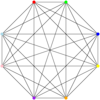
The CLIQUE problem is described as follows: given a graph (a set of vertices and edges) $G$ , does it contain a clique of size $k$ ? A clique of size $k$ is a set of $k$ vertices that are all connected to one another. For instance, this thing below is a clique of size 8. Also note that it does contain cliques of size 1 (single vertex), 2 (an edge), 3 (a triangle), 4, 5, 6, 7, since we can find sets of vertices of that size that are all connected to one another.

Let us reduce 3-SAT to that problem; since 3-SAT is NP-hard, CLIQUE will then be proven to be NP-hard as well. CLIQUE is in NP, because if I provide you with $k$ vertices, it’s possible to check that all these vertices are indeed connected to one another. So, if CLIQUE is NP-hard, CLIQUE is NP-complete.

To start with my reduction, I pick an arbitrary 3-SAT formula – more precisely, a 3-CNF-SAT formula (I explained the meaning of this in my post on SAT), which is a formula that has that look:

$(x_1 \vee x_2 \vee x_3) \wedge (\bar x_2 \vee x_4 \vee \bar x_5) \wedge (x_1 \vee \bar x_2 \vee \bar x_3) \wedge ...$

that is to say, a set of $m$ clauses connected by AND and composed of 3 literals connected by OR.

From there, we’re creating a graph that contains $3m$ vertices. Every vertex corresponds to a literal of the formula; vertices can be duplicated. For the above formula (truncated before the …), this yields the following vertices :

$x_1, x_2, x_3 ; \bar x_2, \bar x_4, \bar x_5 ; x_1, \bar x_2, \bar x_3$ .

Then, we add edges almost everywhere. We don’t add edges in the “groups” that correspond to the clauses, and we also do not add edges between literals that are not compatible, that is to say inverse of each other. If I have two literals $x_1$ and $\bar x_1$ , I’m not creating an edge between them. For the formula above, this is the graph in question:

And these are the edges that are NOT in the previous graph:

And now that we have that graph, we want to show that the SAT formula can be satisfied if and only if the graph (the first one) has a clique of size $m$ , where $m$ is the number of clauses in the SAT formula. So I need to prove two things:

if the formula can be satisfied, then the graph has a clique of size $m$ ,
if the graph has a clique of size $m$ , then the formula can be satisfied.

Let’s start with the first point. Suppose the formula can be satisfied. This means that we can assign a value to all the variables so that the formula is satisfied. This means that all clauses can be satisfied by this assignment. This also means that, for each clause, there’s a literal with value 1 (either a “positive” literal, for instance $x_1$ if the variable is assigned to 1, or a “negative” literal, for instance $\bar x_1$ , if the variable is assigned to 0). Now remember that we created vertices grouped by “clause”, so for each clause, we can pick the vertex corresponding to that 1-valued literal (and if several literals have value 1 in a clause, we can pick an arbitrary one). Since we pick a vertex by clause, and we have $m$ clauses, we have $m$ vertices. We now want to prove that these $m$ vertices form a clique, which means that there is an edge between every pair of vertices of that set. We constructed the graph such that there is no edge between two vertices of a given clause, and we’re fine there, because we chose exactly one vertex per clause. Moreover, there is no edge between a literal and its negation – we’re also fine there, because we only picked literals that have value 1, and $x_i$ and $\bar x_i$ can’t both have value 1. These are the only conditions for which there is no edge between two vertices; which means that our $m$ vertices are all connected with each other, which yields a clique of size $m$ , which is what we want.

Now, let’s look at the second point: if the graph has a clique of size $m$ , then the formula can be satisfied. Suppose that the graph has a clique of size $m$ . Since the vertices corresponding to the literals of a clause are not connected, this means that we have a vertex for each clause. We can give the value 1 to all the literals corresponding to these vertices. We cannot have a clique containing $x_i$ and $\bar x_i$ , because there would be no edge between these two vertices, which goes against the definition of a clique, where all edges are present. So if a clique of size $m$ exists, this means that we found, for each clause, a literal whose value can be 1, and that all of these literals are compatible with each other. And so, we can satisfy the formula corresponding to the graph, which we also wanted to prove.

So, if we can solve CLIQUE in polynomial time, then we can solve 3-SAT in polynomial time; since 3-SAT is NP-hard, CLIQUE is NP-hard, so CLIQUE is NP-complete, which concludes the proof.

Showing that a problem is NP-complete is, in a way, an indicator that the problem in question is difficult, but this needs to be mitigated a lot. For one thing, it does not say anything about a specific instance of the problem. It does not say anything about a specific subset of instances either – let me explain that. If I say that CLIQUE is difficult, it doesn’t mean that, for example, deciding whether a triangle (a clique of size 3) is in a graph is difficult. I can take all sets of 3 vertices, look at whether they form a triangle, and conclude. There are approximately $n^3$ sets of 3 vertices in a graph with $n$ vertices (okay, there’s exactly $\displaystyle \frac{n(n-1)(n-2)}{6}$ – anyway, roughly $n^3$ ), so I can actually decide that in polynomial time (because I’m doing $n^3$ operations which are basically checking if three edges are in a graph). So I can decide 3-CLIQUE in polynomial time. Well, I’m not going to be a millionaire with that, because the CLIQUE problem is wider than just 3. I can also decide 1000-CLIQUE (clique of size 1000) in polynomial time with the same principle. Well, it’s a polynomial of degree 1000, but who cares 😛

But, in the general case, I cannot decide whether a graph over $n$ vertices contains a clique of $\displaystyle \frac{n}{2}$ , or $\displaystyle \frac{n}{10000}$ vertices, or even $\log n$ vertices in polynomial time with this algorithm that looks at all groups of size $k$ (so, here, $k$ would be equal to $\displaystyle \frac{n}{2}$ , $\displaystyle \frac{n}{10000}$ , or $\log n$ ) and that looks at the edges of the group, because that would mean doing roughly $n^{n/2}$ , $n^{n/10000}$ and $n^{\log n}$ operations, respectively, and that in any case it’s not polynomial. And, generally speaking, nobody knows if it’s possible to do that in polynomial time, since CLIQUE is NP-complete and we don’t know if P is equal to NP. Many people think that not, but nobody knows.

Even that does not say anything about the difficulty of a specific instance. If I’m given a graph that contains $\displaystyle \frac{n(n-1)}{2}$ edges for $n$ vertices, then I can decide pretty easily that it does contain a clique of size $\displaystyle \frac{n}{2}$ , $\displaystyle \frac{n}{10000}$ and $\log n$ . That’s because a graph that has $\displaystyle \frac{n(n-1)}{2}$ for $n$ vertices contains all the possible edges for the graph: it’s a clique on $n$ vertices… which means that every subgraph over $k$ vertices, for all $k \leq n$ , is a clique of size $k$ . Same thing if I’m given a graph over $n$ vertices with 0 edge, it’s not going to be hard to say that it doesn’t contain a clique of size $\displaystyle \frac n 2$ .

SAT is also NP-hard, but can solve 2-CNF-SAT instances (where all clauses contain 2 literals) in polynomial, and even linear time. There are also SAT instances that are deemed “easy”, for instance the ones that have only few dependencies between the clauses: we know that we can to solve them, and we even know how (for the people who are interested in what I mean exactly by what I mean by “a few dependencies”, I’m thinking specifically about “the ones that are in the scope of the Lovász Local Lemma“, whose application to SAT is not trivial from the Wikipedia definition, but which might be clearer here).

Generally speaking, it may even be pretty difficult to create NP-hard instances of problems that we cannot solve in polynomial time. By the way, it’s not easy to show that we don’t know how to solve a given instance in polynomial time. We can find instances problem instances that are hard (i.e. require exponential time) for a given algorithm, and easy for another algorithm…

And that’s a bit of what happens in real life: we have instance of problems for which we know that the general case is NP-hard (or worse), and that we still solve without great difficulty. It can be that the problem is “small” (it’s not a huge problem to put an exponential algorithm on a problem of size 4), but it can also be that the problem belongs to an “easy” subset of instances. Considering that an instance of a problem is hard because the general problem is hard, and giving up on it (because we won’t know how to do it) may not be a good idea – it may be that we forgot to consider an easy restriction of the problem!

As usual, “it’s not that simple”. I’ve spent a fair amount of time with theory, and I tend to look at the problems themselves more than at given instances. But it’s sometimes nice to remember that stuff that’s “theoretically hard” can end up being “practically easy” – it’s a nice change from the things that are theoretically easy but that we don’t know how to do practically… 🙂

	Alexandre Franke on SPIEL 2025 in Essen
	Scavenger Hunt round… on Iceland – Day 10
	Scavenger Hunt round… on Iceland – Day 12
	Scavenger Hunt round… on Iceland – Day 6
	Sabbatical report –… on Clair Obscur: Expedition …